Difference between revisions of "Fossil energy resources - COFFEE-TEA"
| Line 4: | Line 4: | ||
}} | }} | ||
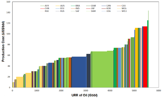
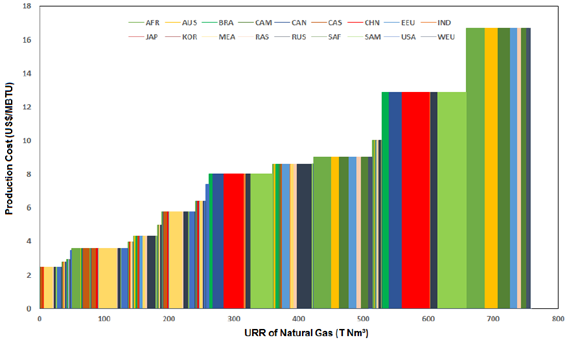
| − | The oil and natural gas supply curve in the COFFEE model were built based on several studies. The data was obtained from the detailed resource assessments in USGS (2000), USGS (2007), WEC (2010) , USGS (2012), WEC (2013) and MCGLADE (2013), detailed technical parameters (such as Enhanced Oil Recovery, or EOR, recovery rates and potential) available in MCGLADE (2013) and ROGNER (1997), and also the cost data from MCGLADE (2013) and IEA (2014), the following data were gathered processed and compiled to determine the supply curve, as shown in <xr id="fig:Oil"/>. | + | The oil and natural gas supply curve in the COFFEE model were built based on several studies. The data was obtained from the detailed resource assessments in USGS (2000), USGS (2007), WEC (2010) , USGS (2012), WEC (2013) and MCGLADE (2013), detailed technical parameters (such as Enhanced Oil Recovery, or EOR, recovery rates and potential) available in MCGLADE (2013) and ROGNER (1997), and also the cost data from MCGLADE (2013) and IEA (2014), the following data were gathered processed and compiled to determine the supply curve, as shown in <xr id="fig:Oil"/> and <xr id="fig:Gas"/>. |
<figure id="fig:Oil"> | <figure id="fig:Oil"> | ||
| Line 10: | Line 10: | ||
</figure>. | </figure>. | ||
| − | A coal resource assessment profile was also developed to check this availability. In the model, the categories defined for coal are betuminous, sub-betuminous, and lignite, all of them split in surface or mining availability for each region. The main sources of information for developing a specific supply curve were ROGNER (1997), as it deals with hydrocarbons in general, WEC (2013), IEA (2014), MCGLADE AND EKINS (2015) and GMI (2015). These studies were used to the estimate the methane content for every coal resource category. | + | <figure id="fig:Gas"> |
| + | [[File:gas.png|600px|thumb|<caption>Natural gas supply curve detailing each regional resource</caption>]] | ||
| + | </figure>. | ||
| + | |||
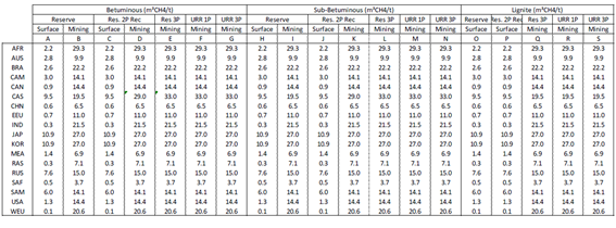
| + | A coal resource assessment profile was also developed to check this availability. In the model, the categories defined for coal are betuminous, sub-betuminous, and lignite, all of them split in surface or mining availability for each region. The main sources of information for developing a specific supply curve were ROGNER (1997), as it deals with hydrocarbons in general, WEC (2013), IEA (2014), MCGLADE AND EKINS (2015) and GMI (2015). These studies were used to the estimate the methane content for every coal resource category (<xr id="fig:Coal"/>). | ||
| + | |||
| + | <figure id="fig:Coal"> | ||
| + | [[File:coal.png|600px|thumb|<caption>Methane content for every region and resource category</caption>]] | ||
| + | </figure>. | ||
Revision as of 17:19, 25 February 2019
| Corresponding documentation | |
|---|---|
| Previous versions | |
| Model information | |
| Model link | |
| Institution | COPPE/UFRJ (Cenergia), Brazil, http://www.cenergialab.coppe.ufrj.br/. |
| Solution concept | General equilibrium (closed economy) |
| Solution method | The COFFEE model is solved through Linear Programming (LP). The TEA model is formulated as a mixed complementary problem (MCP) and is solved through Mathematical Programming System for General Equilibrium -- MPSGE within GAMS using the PATH solver. |
| Anticipation | |
The oil and natural gas supply curve in the COFFEE model were built based on several studies. The data was obtained from the detailed resource assessments in USGS (2000), USGS (2007), WEC (2010) , USGS (2012), WEC (2013) and MCGLADE (2013), detailed technical parameters (such as Enhanced Oil Recovery, or EOR, recovery rates and potential) available in MCGLADE (2013) and ROGNER (1997), and also the cost data from MCGLADE (2013) and IEA (2014), the following data were gathered processed and compiled to determine the supply curve, as shown in Figure 1 and Figure 2.
.
.
A coal resource assessment profile was also developed to check this availability. In the model, the categories defined for coal are betuminous, sub-betuminous, and lignite, all of them split in surface or mining availability for each region. The main sources of information for developing a specific supply curve were ROGNER (1997), as it deals with hydrocarbons in general, WEC (2013), IEA (2014), MCGLADE AND EKINS (2015) and GMI (2015). These studies were used to the estimate the methane content for every coal resource category (Figure 3).
.
References
- ^ Christophe E McGlade(2014). Uncertainties in the outlook for oil and gas. Retrieved from http://discovery.ucl.ac.uk/1418473/
- a b | | Hans-Holger Rogner (1997). An assessment of world hydrocarbon resources. Annual review of energy and the environment, 22 (1), 217-262.
- ^ IEA(2014). World Energy Outlook 2014. Retrieved from https://www.iea.org/publications/freepublications/publication/WEO2014.pdf


