Snapshot of - BLUES

Archive of BLUES, version: 1.0

Reference card - BLUES

The reference card is a clearly defined description of model features. The numerous options have been organized into a limited amount of default and model specific (non default) options. In addition some features are described by a short clarifying text.

Legend:

• not implemented
• implemented
• implemented (not default option)

About

Name and version

BLUES 1.0

Model link

https://www.nature.com/articles/s41558-018-0213-y

Institution

COPPE/UFRJ (Cenergia), Brazil, http://www.cenergialab.coppe.ufrj.br/.

Documentation

BLUES documentation consists of a referencecard and detailed model documentation

Process state

published

Model scope and methods

Model documentation: Model scope and methods - BLUES

Model type

• Integrated assessment model
• Energy system model
• CGE
• CBA-integrated assessment model

Geographical scope

• Global
• Regional

Solution concept

• Partial equilibrium (price elastic demand)
• Partial equilibrium (fixed demand)
• General equilibrium (closed economy)

Note: BLUES is partial equilibrium energy-land system model, with integration with the TEA model (CGE model).

Solution horizon

• Recursive dynamic (myopic)
• Intertemporal optimization (foresight)

Solution method

• Simulation
• Optimization

Temporal dimension

Base year:2010, time steps:5 year, horizon: 2050

Spatial dimension

Number of regions:5

Time discounting type

• Discount rate exogenous
• Discount rate endogenous

Policies

• Emission tax
• Emission pricing
• Cap and trade
• Fuel taxes
• Fuel subsidies
• Feed-in-tariff
• Portfolio standard
• Capacity targets
• Emission standards
• Energy efficiency standards
• Agricultural producer subsidies
• Agricultural consumer subsidies
• Land protection
• Pricing carbon stocks

Socio-economic drivers

Model documentation: Socio-economic drivers - BLUES

Population

• Yes (exogenous)
• Yes (endogenous)

Population age structure

• Yes (exogenous)
• Yes (endogenous)

Education level

• Yes (exogenous)
• Yes (endogenous)

Urbanization rate

• Yes (exogenous)
• Yes (endogenous)

GDP

• Yes (exogenous)
• Yes (endogenous)

Income distribution

• Yes (exogenous)
• Yes (endogenous)

Employment rate

• Yes (exogenous)
• Yes (endogenous)

Labor productivity

• Yes (exogenous)
• Yes (endogenous)

Total factor productivity

• Yes (exogenous)
• Yes (endogenous)

Autonomous energy efficiency improvements

• Yes (exogenous)
• Yes (endogenous)

Macro-economy

Model documentation: Macro-economy - BLUES

Economic sector

Industry

• Yes (physical)
• Yes (economic)
• Yes (physical & economic)

Energy

• Yes (physical)
• Yes (economic)
• Yes (physical & economic)

Transportation

• Yes (physical)
• Yes (economic)
• Yes (physical & economic)

Residential and commercial

• Yes (physical)
• Yes (economic)
• Yes (physical & economic)

Agriculture

• Yes (physical)
• Yes (economic)
• Yes (physical & economic)

Forestry

• Yes (physical)
• Yes (economic)
• Yes (physical & economic)

Macro-economy

Trade

• Coal
• Oil
• Gas
• Uranium
• Electricity
• Bioenergy crops
• Food crops
• Capital
• Emissions permits
• Non-energy goods

Cost measures

• GDP loss
• Welfare loss
• Consumption loss
• Area under MAC
• Energy system cost mark-up

Categorization by group

• Income
• Urban - rural
• Technology adoption
• Age
• Gender
• Education level
• Household size

Institutional and political factors

• Early retirement of capital allowed
• Interest rates differentiated by country/region
• Regional risk factors included
• Technology costs differentiated by country/region
• Technological change differentiated by country/region
• Behavioural change differentiated by country/region
• Constraints on cross country financial transfers

Resource use

Coal

• Yes (fixed)
• Yes (supply curve)
• Yes (process model)

Conventional Oil

• Yes (fixed)
• Yes (supply curve)
• Yes (process model)

Unconventional Oil

• Yes (fixed)
• Yes (supply curve)
• Yes (process model)

Conventional Gas

• Yes (fixed)
• Yes (supply curve)
• Yes (process model)

Unconventional Gas

• Yes (fixed)
• Yes (supply curve)
• Yes (process model)

Uranium

• Yes (fixed)
• Yes (supply curve)
• Yes (process model)

Bioenergy

• Yes (fixed)
• Yes (supply curve)
• Yes (process model)

Water

• Yes (fixed)
• Yes (supply curve)
• Yes (process model)

Raw Materials

• Yes (fixed)
• Yes (supply curve)
• Yes (process model)

Land

• Yes (fixed)
• Yes (supply curve)
• Yes (process model)

Technological change

Energy conversion technologies

• No technological change
• Exogenous technological change
• Endogenous technological change

Energy End-use

• No technological change
• Exogenous technological change
• Endogenous technological change

Material Use

• No technological change
• Exogenous technological change
• Endogenous technological change

Agriculture (tc)

• No technological change
• Exogenous technological change
• Endogenous technological change

Energy

Model documentation: Energy - BLUES

Energy technology substitution

Energy technology choice

• No discrete technology choices
• Logit choice model
• Production function
• Linear choice (lowest cost)
• Lowest cost with adjustment penalties

Energy technology substitutability

• Mostly high substitutability
• Mostly low substitutability
• Mixed high and low substitutability

Energy technology deployment

• Expansion and decline constraints
• System integration constraints

Energy

Electricity technologies

• Coal w/o CCS
• Coal w/ CCS
• Gas w/o CCS
• Gas w/ CCS
• Oil w/o CCS
• Oil w/ CCS
• Bioenergy w/o CCS
• Bioenergy w/ CCS
• Geothermal power
• Nuclear power
• Solar power
• Solar power-central PV
• Solar power-distributed PV
• Solar power-CSP
• Wind power
• Wind power-onshore
• Wind power-offshore
• Hydroelectric power
• Ocean power
• Hydrokinetic

Hydrogen production

• Coal to hydrogen w/o CCS
• Coal to hydrogen w/ CCS
• Natural gas to hydrogen w/o CCS
• Natural gas to hydrogen w/ CCS
• Oil to hydrogen w/o CCS
• Oil to hydrogen w/ CCS
• Biomass to hydrogen w/o CCS
• Biomass to hydrogen w/ CCS
• Nuclear thermochemical hydrogen
• Solar thermochemical hydrogen
• Electrolysis

Refined liquids

• Coal to liquids w/o CCS
• Coal to liquids w/ CCS
• Gas to liquids w/o CCS
• Gas to liquids w/ CCS
• Bioliquids w/o CCS
• Bioliquids w/ CCS
• Oil refining

Refined gases

• Coal to gas w/o CCS
• Coal to gas w/ CCS
• Oil to gas w/o CCS
• Oil to gas w/ CCS
• Biomass to gas w/o CCS
• Biomass to gas w/ CCS

Heat generation

• Coal heat
• Natural gas heat
• Oil heat
• Biomass heat
• Geothermal heat
• Solarthermal heat
• CHP (coupled heat and power)

Grid Infra Structure

Electricity

• Yes (aggregate)
• Yes (spatially explicit)

Gas

• Yes (aggregate)
• Yes (spatially explicit)

Heat

• Yes (aggregate)
• Yes (spatially explicit)

CO2

• Yes (aggregate)
• Yes (spatially explicit)

Hydrogen

• Yes (aggregate)
• Yes (spatially explicit)

Energy end-use technologies

Passenger transportation

• Passenger trains
• Buses
• Light Duty Vehicles (LDVs)
• Electric LDVs
• Hydrogen LDVs
• Hybrid LDVs
• Gasoline LDVs
• Diesel LDVs
• Passenger aircrafts

Freight transportation

• Freight trains
• Heavy duty vehicles
• Freight aircrafts
• Freight ships

Industry

• Steel production
• Aluminium production
• Cement production
• Petrochemical production
• Paper production
• Plastics production
• Pulp production

Residential and commercial

• Space heating
• Space cooling
• Cooking
• Refrigeration
• Washing
• Lighting

Land-use

Model documentation: Land-use - BLUES

Land cover

• Cropland
• Cropland irrigated
• Cropland food crops
• Cropland feed crops
• Cropland energy crops
• Forest
• Managed forest
• Natural forest
• Pasture
• Shrubland
• Built-up area
• Pasture HighCapacity
• Pasture LowCapacity
• IntegratedSystems
• DoubleCrop
• ILPF

Agriculture and forestry demands

• Agriculture food
• Agriculture food crops
• Agriculture food livestock
• Agriculture feed
• Agriculture feed crops
• Agriculture feed livestock
• Agriculture non-food
• Agriculture non-food crops
• Agriculture non-food livestock
• Agriculture bioenergy
• Agriculture residues
• Forest industrial roundwood
• Forest fuelwood
• Forest residues

Agricultural commodities

• Wheat
• Rice
• Other coarse grains
• Oilseeds
• Sugar crops
• Ruminant meat
• Non-ruminant meat and eggs
• Dairy products

Emission, climate and impacts

Model documentation: Emissions - BLUES, Climate - BLUES, Non-climate sustainability dimension - BLUES

Greenhouse gases

• CO2 fossil fuels
• CO2 cement
• CO2 land use
• CH4 energy
• CH4 land use
• CH4 other
• N2O energy
• N2O land use
• N2O other
• CFCs
• HFCs
• SF6
• PFCs

Pollutants

• CO energy
• CO land use
• CO other
• NOx energy
• NOx land use
• NOx other
• VOC energy
• VOC land use
• VOC other
• SO2 energy
• SO2 land use
• SO2 other
• BC energy
• BC land use
• BC other
• OC energy
• OC land use
• OC other
• NH3 energy
• NH3 land use
• NH3 other
• PM energy
• PM land use
• PM other

Climate indicators

• Concentration: CO2
• Concentration: CH4
• Concentration: N2O
• Concentration: Kyoto gases
• Radiative forcing: CO2
• Radiative forcing: CH4
• Radiative forcing: N2O
• Radiative forcing: F-gases
• Radiative forcing: Kyoto gases
• Radiative forcing: aerosols
• Radiative forcing: land albedo
• Radiative forcing: AN3A
• Radiative forcing: total
• Temperature change
• Sea level rise
• Ocean acidification

Carbon dioxide removal

• Bioenergy with CCS
• Reforestation
• Afforestation
• Soil carbon enhancement
• Direct air capture
• Enhanced weathering

Climate change impacts

• Agriculture
• Energy supply
• Energy demand
• Economic output
• Built capital
• Inequality

Co-Linkages

• Energy security: Fossil fuel imports & exports (region)
• Energy access: Household energy consumption
• Air pollution & health: Source-based aerosol emissions
• Air pollution & health: Health impacts of air Pollution
• Food access
• Water availability
• Biodiversity

Model Documentation - BLUES

The Brazilian Land Use and Energy System (BLUES) model is a perfect-foresight, least-cost optimization model for Brazil. It chooses the energy system configuration with the least total system cost over the entire time horizon of the study, in this case 2010 to 2050. The model minimizes costs of the entire energy system, including electricity generation, agriculture, industry, transport and the buildings sectors. BLUES finds optimized mixes for the energy system as a whole, rather than evaluating sectorial optimal solutions. It includes CO2, CH4 and N2O emissions associated with land use, agriculture and livestock, fugitive emissions, fuel combustion, industrial processes and waste treatment.

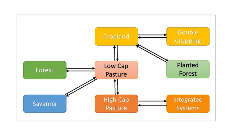
BLUES has six native regions. One main overarching region into which five sub-regions are nested following the geopolitical division of the country. The energy system is represented in detail across sectors, with over 1500 technologies available in and customized for each of its six native regions. The representation of the land-use system includes forests, savannas, low- and high-capacity pastures, integrated systems, cropland, double cropping, planted forests, and protected areas. Cropland is made up of Land useis also regionalized and customized for each subregion, with yields and costs varying from region to region. Demand is exogenous but endogenous energy efficiency measures permit demand responses through technological options.

2) Socio-economic drivers - BLUES

Population and GDP (MER) are the main exogenous socio-economic drivers behind demand projections in the Reference scenario implemented in BLUES. Demand projections are derived from GDP and population projections through econometric and regression techniques.

2.1) Population - BLUES

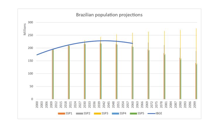
Population projection through 2050 was taken from the Instituto Brasileiro de Geografia e Estatistica (IBGE 2016). It compares well with the projection for SSP2 (KC & Lutz 2017), as shown in the figure below.

Population projections for Brazil from IBGE and SSPs/caption>

References

IBGE (2016). Projeção da População do Brasil por sexo e idade: 2000-2060. Instituto Brasileiro de Geografia e Estatistica. Accessed online on July 1 2015 at https://ww2.ibge.gov.br/home/estatistica/populacao/projecao_da_populacao/2013/default.shtm

KC, S., Lutz, W., 2017. The human core of the shared socioeconomic pathways: Population scenarios by age, sex and level of education for all countries to 2100. Glob. Environ. Chang. 42, 181–192. doi:10.1016/j.gloenvcha.2014.06.004

2.2) Economic activity - BLUES

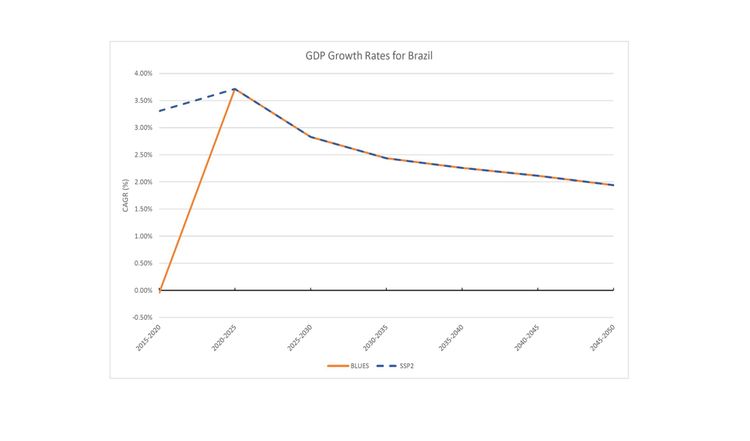
GDP growth rate projections are based largely on SSPs projections (Dellink et al 2015), with adjustments made for the short-term to reflect current economic activity in Brazil. Short-term projections through 2020 are based on The Focus Bulletin published by the Brazilian Central Bank (BCB 2017). The GDP projection of the Reference scenario in BLUES is shown in the figure below.

Population projections for Brazil from IBGE and SSPs/caption>

References

BCB. (2017). Sistema de Expectativas de Mercado. Retrieved September 01, 2017, from https://www3.bcb.gov.br/expectativas/publico/consulta/serieestatisticas

Dellink, R., Chateau, J., Lanzi, E., Magné, B., 2015. Long-term economic growth projections in the Shared Socioeconomic Pathways. Glob. Environ. Chang. IN PRESS, 1–15. doi:10.1016/j.gloenvcha.2015.06.004

4) Energy - BLUES

Techno-economic parameters that form the input deck of COPPE-MSB were derived from various sources (Koberle et al., 2015; Nogueira et al., 2014; J Portugal-Pereira et al., 2016; Soria et al., 2015). Techno-economic input parameters of IAMs in general, and also of COPPE-MSB, include specific investment costs (CAPEX, in US$/kW), construction times (years), conversion efficiency (%), and any technical or economic specifications that may be required to appropriately model the performance of an energy technology (investment and O&M costs, minimum utilization time, inputs and outputs, auxiliary inputs and secondary outputs among others).

5) Land-use - BLUES

Land Use classes

A representative set of distinct land use classes were chosen to optimize representation and minimize computational requirements in the MESSAGE framework. The starting point were the CSR-UFMG maps uso_da_terra_2013 representing land use in 2013 as allocated by the land use model OTIMIZAGRO (http://maps.csr.ufmg.br/). The map represents the cultivated area of 14 crops, double crop areas, planted forests and pastures, plus the natural remnants of forests and savannas, both inside and outside of protected areas (Soares-Filho et al., 2016). It also shows urban areas and water bodies which were used to create an exclusion mask for agricultural activities. These land use class were aggregated for our purposes according into 9 base-year land use classes:

Cropland, Double crop areas, Pastures, Planted Forests, Savannas, Savannas in Protected Areas, Forests, Forests in Protected Areas.

Pastures were then divided into two categories of grazing intensity: Low-capacity pastures with <0.8 AU/ha and High-capacity pastures with >0.8 AU/ha.

The spatial allocation and area calculation of the two classes of pastures was derived from the "Lotação Bovina no Brasil" map from LAPIG (http://maps.lapig.iesa.ufg.br/lapig.html).

To these base-year LU classes was added the Integrated Systems LU class. It represents Crop-Livestock-Forest Integrated Agricultural Systems and is not represented in the initial area allocation as it occupied a negligible area in the base year. However, this production system has gained much attention in recent years and is one of the cornerstones of future intensification of Brazilian agriculture, and an important mitigation measure in the Brazilian Low Carbon Agriculture Plan (MAPA, 2011).

5.3) Land-use change - BLUES

Land Use Transitions

The figure below shows the allowed land use transitions in BLUES. Note that a unit area may undergo more than one transition in each time step.

BLUES Land Use Transitions diagram