Snapshot of - GRACE
Archive of GRACE, version: 2018
Reference card - GRACE
The reference card is a clearly defined description of model features. The numerous options have been organized into a limited amount of default and model specific (non default) options. In addition some features are described by a short clarifying text.
Legend:
- not implemented
- implemented
- implemented (not default option)
About
Name and version
GRACE 2018
Institution
Center for International Climate Research (CICERO), Norway, https://cicero.oslo.no/en.
Documentation
GRACE documentation consists of a referencecard and detailed model documentation
Process state
under review
Model scope and methods
Model documentation: Model scope and methods - GRACE
Model type
- Integrated assessment model
- Energy system model
- CGE
- CBA-integrated assessment model
Geographical scope
- Global
- Regional
Objective
The model aims primarily to estimating how economic indicators defined in the national accounts interact with climate-related factors. for example, climate policies are represented by e.g. quotas or taxes on emissions, to show the economic consequences in world regions under projections.
Solution concept
- Partial equilibrium (price elastic demand)
- Partial equilibrium (fixed demand)
- General equilibrium (closed economy)
Solution horizon
- Recursive dynamic (myopic)
- Intertemporal optimization (foresight)
Solution method
- Simulation
- Optimization
- Recursive dynamic solution method
Temporal dimension
Base year:2014, time steps:yearly, horizon:
Spatial dimension
Number of regions:up to 140.
Time discounting type
- Discount rate exogenous
- Discount rate endogenous
Policies
- Emission tax
- Emission pricing
- Cap and trade
- Fuel taxes
- Fuel subsidies
- Feed-in-tariff
- Portfolio standard
- Capacity targets
- Emission standards
- Energy efficiency standards
- Agricultural producer subsidies
- Agricultural consumer subsidies
- Land protection
- Pricing carbon stocks
- Adaptation, climate change impact
Socio-economic drivers
Model documentation: Socio-economic drivers - GRACE
Population
- Yes (exogenous)
- Yes (endogenous)
Population age structure
- Yes (exogenous)
- Yes (endogenous)
Education level
- Yes (exogenous)
- Yes (endogenous)
Urbanization rate
- Yes (exogenous)
- Yes (endogenous)
GDP
- Yes (exogenous)
- Yes (endogenous)
Income distribution
- Yes (exogenous)
- Yes (endogenous)
Employment rate
- Yes (exogenous)
- Yes (endogenous)
Labor productivity
- Yes (exogenous)
- Yes (endogenous)
Total factor productivity
- Yes (exogenous)
- Yes (endogenous)
Autonomous energy efficiency improvements
- Yes (exogenous)
- Yes (endogenous)
Macro-economy
Model documentation: Macro-economy - GRACE
Economic sector
Industry
- Yes (physical)
- Yes (economic)
- Yes (physical & economic)
Energy
- Yes (physical)
- Yes (economic)
- Yes (physical & economic)
Transportation
- Yes (physical)
- Yes (economic)
- Yes (physical & economic)
Residential and commercial
- Yes (physical)
- Yes (economic)
- Yes (physical & economic)
Agriculture
- Yes (physical)
- Yes (economic)
- Yes (physical & economic)
Forestry
- Yes (physical)
- Yes (economic)
- Yes (physical & economic)
Other economic sector
- Services (economic)
Macro-economy
Trade
- Coal
- Oil
- Gas
- Uranium
- Electricity
- Bioenergy crops
- Food crops
- Capital
- Emissions permits
- Non-energy goods
- Agriculture
- Consumer Goods Industries
- Livestock products
- Manufactures
- Services
- Refined Liquid Fuels
Cost measures
- GDP loss
- Welfare loss
- Consumption loss
- Area under MAC
- Energy system cost mark-up
- Equivalent Variation
Categorization by group
- Income
- Urban - rural
- Technology adoption
- Age
- Gender
- Education level
- Household size
Institutional and political factors
- Early retirement of capital allowed
- Interest rates differentiated by country/region
- Regional risk factors included
- Technology costs differentiated by country/region
- Technological change differentiated by country/region
- Behavioural change differentiated by country/region
- Constraints on cross country financial transfers
Resource use
Coal
- Yes (fixed)
- Yes (supply curve)
- Yes (process model)
Conventional Oil
- Yes (fixed)
- Yes (supply curve)
- Yes (process model)
Unconventional Oil
- Yes (fixed)
- Yes (supply curve)
- Yes (process model)
Conventional Gas
- Yes (fixed)
- Yes (supply curve)
- Yes (process model)
Unconventional Gas
- Yes (fixed)
- Yes (supply curve)
- Yes (process model)
Uranium
- Yes (fixed)
- Yes (supply curve)
- Yes (process model)
Bioenergy
- Yes (fixed)
- Yes (supply curve)
- Yes (process model)
Water
- Yes (fixed)
- Yes (supply curve)
- Yes (process model)
Raw Materials
- Yes (fixed)
- Yes (supply curve)
- Yes (process model)
Land
- Yes (fixed)
- Yes (supply curve)
- Yes (process model)
Technological change
Energy conversion technologies
- No technological change
- Exogenous technological change
- Endogenous technological change
Energy End-use
- No technological change
- Exogenous technological change
- Endogenous technological change
Material Use
- No technological change
- Exogenous technological change
- Endogenous technological change
Agriculture (tc)
- No technological change
- Exogenous technological change
- Endogenous technological change
Energy
Model documentation: Energy - GRACE
Behaviour
Producers maximize profit and consumers maximize utility.
Energy technology substitution
Energy technology choice
- No discrete technology choices
- Logit choice model
- Production function
- Linear choice (lowest cost)
- Lowest cost with adjustment penalties
- Nested CES function
Energy technology substitutability
- Mostly high substitutability
- Mostly low substitutability
- Mixed high and low substitutability
Energy technology deployment
- Expansion and decline constraints
- System integration constraints
Energy
Electricity technologies
- Coal w/o CCS
- Coal w/ CCS
- Gas w/o CCS
- Gas w/ CCS
- Oil w/o CCS
- Oil w/ CCS
- Bioenergy w/o CCS
- Bioenergy w/ CCS
- Geothermal power
- Nuclear power
- Solar power
- Solar power-central PV
- Solar power-distributed PV
- Solar power-CSP
- Wind power
- Wind power-onshore
- Wind power-offshore
- Hydroelectric power
- Ocean power
Hydrogen production
- Coal to hydrogen w/o CCS
- Coal to hydrogen w/ CCS
- Natural gas to hydrogen w/o CCS
- Natural gas to hydrogen w/ CCS
- Oil to hydrogen w/o CCS
- Oil to hydrogen w/ CCS
- Biomass to hydrogen w/o CCS
- Biomass to hydrogen w/ CCS
- Nuclear thermochemical hydrogen
- Solar thermochemical hydrogen
- Electrolysis
Refined liquids
- Coal to liquids w/o CCS
- Coal to liquids w/ CCS
- Gas to liquids w/o CCS
- Gas to liquids w/ CCS
- Bioliquids w/o CCS
- Bioliquids w/ CCS
- Oil refining
Refined gases
- Coal to gas w/o CCS
- Coal to gas w/ CCS
- Oil to gas w/o CCS
- Oil to gas w/ CCS
- Biomass to gas w/o CCS
- Biomass to gas w/ CCS
Heat generation
- Coal heat
- Natural gas heat
- Oil heat
- Biomass heat
- Geothermal heat
- Solarthermal heat
- CHP (coupled heat and power)
Grid Infra Structure
Electricity
- Yes (aggregate)
- Yes (spatially explicit)
Gas
- Yes (aggregate)
- Yes (spatially explicit)
Heat
- Yes (aggregate)
- Yes (spatially explicit)
CO2
- Yes (aggregate)
- Yes (spatially explicit)
Hydrogen
- Yes (aggregate)
- Yes (spatially explicit)
Energy end-use technologies
Passenger transportation
- Passenger trains
- Buses
- Light Duty Vehicles (LDVs)
- Electric LDVs
- Hydrogen LDVs
- Hybrid LDVs
- Gasoline LDVs
- Diesel LDVs
- Passenger aircrafts
Freight transportation
- Freight trains
- Heavy duty vehicles
- Freight aircrafts
- Freight ships
Industry
- Steel production
- Aluminium production
- Cement production
- Petrochemical production
- Paper production
- Plastics production
- Pulp production
Residential and commercial
- Space heating
- Space cooling
- Cooking
- Refrigeration
- Washing
- Lighting
Land-use
Model documentation: Land-use - GRACE
Land cover
- Cropland
- Cropland irrigated
- Cropland food crops
- Cropland feed crops
- Cropland energy crops
- Forest
- Managed forest
- Natural forest
- Pasture
- Shrubland
- Built-up area
Agriculture and forestry demands
- Agriculture food
- Agriculture food crops
- Agriculture food livestock
- Agriculture feed
- Agriculture feed crops
- Agriculture feed livestock
- Agriculture non-food
- Agriculture non-food crops
- Agriculture non-food livestock
- Agriculture bioenergy
- Agriculture residues
- Forest industrial roundwood
- Forest fuelwood
- Forest residues
Agricultural commodities
- Wheat
- Rice
- Other coarse grains
- Oilseeds
- Sugar crops
- Ruminant meat
- Non-ruminant meat and eggs
- Dairy products
Emission, climate and impacts
Model documentation: Emissions - GRACE, Climate - GRACE, Non-climate sustainability dimension - GRACE
Greenhouse gases
- CO2 fossil fuels
- CO2 cement
- CO2 land use
- CH4 energy
- CH4 land use
- CH4 other
- N2O energy
- N2O land use
- N2O other
- CFCs
- HFCs
- SF6
- PFCs
Pollutants
- CO energy
- CO land use
- CO other
- NOx energy
- NOx land use
- NOx other
- VOC energy
- VOC land use
- VOC other
- SO2 energy
- SO2 land use
- SO2 other
- BC energy
- BC land use
- BC other
- OC energy
- OC land use
- OC other
- NH3 energy
- NH3 land use
- NH3 other
Climate indicators
- Concentration: CO2
- Concentration: CH4
- Concentration: N2O
- Concentration: Kyoto gases
- Radiative forcing: CO2
- Radiative forcing: CH4
- Radiative forcing: N2O
- Radiative forcing: F-gases
- Radiative forcing: Kyoto gases
- Radiative forcing: aerosols
- Radiative forcing: land albedo
- Radiative forcing: AN3A
- Radiative forcing: total
- Temperature change
- Sea level rise
- Ocean acidification
Carbon dioxide removal
- Bioenergy with CCS
- Reforestation
- Afforestation
- Soil carbon enhancement
- Direct air capture
- Enhanced weathering
Climate change impacts
- Agriculture
- Energy supply
- Energy demand
- Economic output
- Built capital
- Inequality
- Extreme events
- labor productivity
Co-Linkages
- Energy security: Fossil fuel imports & exports (region)
- Energy access: Household energy consumption
- Air pollution & health: Source-based aerosol emissions
- Air pollution & health: Health impacts of air Pollution
- Food access
- Water availability
- Biodiversity
Model Documentation - GRACE
The model for Global Responses to Anthropogenic Change in the Environment (GRACE) is a multi-sector, multi-regional, recursively dynamic global computable general equilibrium model (CGE) written in GAMS and based on GTAP database. The initial version of the model was developed at CICERO by Aaheim and Rive (2005) for long-term economic analysis of climate change impacts and greenhouse gas abatement policy. It was designed to allow for additional modules for analysis, including emissions permit trading and climate impacts on economic sectors.
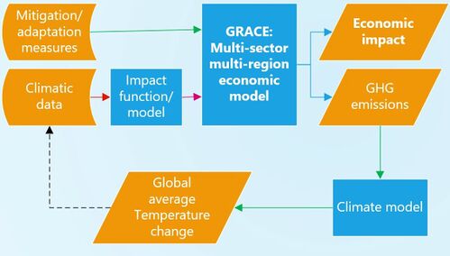
Coupled with an atmospheric model, the model can also be used for integrated assessment modelling of the climate and economy. Since then several versions have been developed by updating data and certain modules for various studies. A recent description of the model is available here.
1) Model scope and methods - GRACE
GRACE is a global recursive dynamic CGE model developed to show the consequences of actions taken to mitigate climate change, and the impacts of the resulting climatic changes on the economic development in selected countries or regions of the world. The model calculates emissions of CO2 and other key greenhouse gases from economic activities, and integrates impacts of climate change, which allows for assessments of the economic consequences of climate projections. The model is programmed and solved on yearly basis in GAMS and uses the GTAP database, which comprises national accounts data for about 60 sectors in 140 world regions, most of them countries. GRACE is seldom run with more than 15 sectors and 15 regions, but aggregation of sectors and regions is flexible and easy to change. Thereby, the model can be used flexibly to focus on specific sectors or regions, depending on the research question.
1.1) Model concept, solver and details - GRACE
GRACE is a global recursive dynamic computable general equilibrium model with multi-regions and multi-sectors. The model is written in GAMS and solved by the solver PATH of GAMS.
1.3) Temporal dimension - GRACE
GRACE is calibrated around a base year (2014 in Nov. 2020). The base year is updated following the latest GTAP database. Then the model can be solved yearly until a future year, such as 2050 and 2100 by updating external variables every year.
1.4) Spatial dimension - GRACE
GRACE covers the whole world. the geographic dimension rely on the data availability. Normally the model aggregate countries into around 15 regions depending on the research demand.
1.5) Policy - GRACE
GRACE can simulate effects of policies of climate mitigation (e.g. carbon tax, carbon market, renewable subsidy, and energy efficiency improvement), climate adaptation measures (e.g. substitution between goods/resources and market responses), climate impact (e.g. climate change impact on crop production and forest growth). the policy options targeting on specific sectors can be introduced in GRACE as it is a multi-sectoral model.
2) Socio-economic drivers - GRACE
Economic growth is driven by investments, population growth, technological change and the availability of natural resources. Labour force growth is exogenously determined in the model and calibrated based on some population projection (e.g., World Bank). In the reference scenario, the real Gross Domestic Product (GDP) is exogenous and calibrated based on some economic growth projection (e.g., World Bank or OECD) by making labour productivity endogenous, i.e., a labour-augmenting technical change. Alternatively, the economic growth in the reference scenario could be calibrated by making total factor productivity endogenous (i.e., labour and capital). In policy simulations, factor endowment is scaled by the calibrated parameters of factor productivity and real GDP is endogenously determined within the model.
2.1) Population - GRACE
Population in GRACE is exogenous based on latest World Population Prospects data released by UNPD. Labor supply by region depends on population size, age, and labor paticipation rate.
2.2) Economic activity - GRACE
GRACE can consider up to 65 production sectors based on the GTAP database v. 10. The model also distinguish private consumption, public consumption, and investments. The bilateral trade is also modeled at sectoral level. Capital assets are allowed to move from one region to another while labor supply and natural resources are immobile across regions.
3) Macro-economy - GRACE
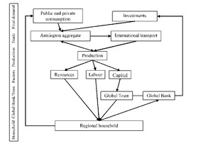
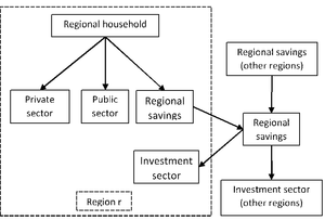
Figures 1 and 2 illustrate the circular flow of payments among the main components of the model, which explicitly depicts interactions between commodity and factor markets as well as interactions among regions. The Regional Household, which represents private households and government in each region, receives the payments from supplying primary factors. The income of the Regional Household is spent on private and public consumption, and savings.
The Global Bank collects savings from all regions and then provides investments to regions so that the expected return to capital equalises among regions. The Global Trust collects the earnings from installed capital and distributes them among regions, given the assumption of perfect capital mobility. Firms use primary factors and intermediates to produce goods and services. Domestic and imported commodities build the so-called Armington aggregate, which is then distributed among private and public consumption and investments.
3.1) Production system and representation of economic sectors - GRACE
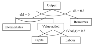
Firms are assumed to supply goods and services to maximise their subject to production technologies in perfect competitive markets. Production technologies are described by nested separable constant elasticity of substitution (CES) functions (see below), and inputs are divided into primary input factors (i.e., labour, capital and resources) and intermediate inputs from each sector. Output and the use of all input factors are subject to taxation, reported in the database. Production of primary energy includes natural resources as a sector-specific production factor, with a fixed supply.
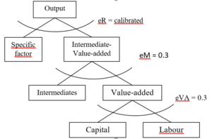
Two forms of the nested CES functions are adopted by the core version of the GRACE model. Figure 2.3 illustrates the structure of the functional forms for production of primary energy – crude oil, coal, and gas. The parameters starting with small letter “e” indicate the elasticities of substitution (the same for figures illustrating structures of nested functions below). At the top-level, output is described by a standard CES function of the value-added-intermediates aggregate and the natural resource. The substitution elasticity at the top-level as well as the value share of natural resource determine the price elasticity of supply of fossil fuels. In the basic version of the GRACE model, this substitution elasticity is set to 0.3. At the second level, the value-added-intermediates aggregate is depicted by a Leontief function (with no substitution) of intermediates and the value-added aggregate. The value-added aggregate is a standard CES function of capital and labour. The substitution elasticity between capital and labour is another important parameter, which determines technological flexibilities in production. The empirical literature typically rejects the hypothesis of a Cobb-Douglas function, where the substitution elasticity between capital and labour equals 1, and shows that the elasticity tends to be less than unity (Arrow et al., 1961). In the core version of the GRACE model, we assume a substitution elasticity of 0.3.
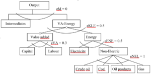
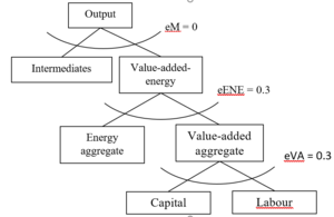
The other form of production functions illustrated in Figure 2.4 is for production of goods/services other than primary energy – crude oil, coal, and gas. Output is described assuming no substitution (Leontief function) between intermediates and the value-added-energy aggregate. At the second level, the value-added-energy aggregate is a standard CES function of the energy aggregate and the value-added aggregate, with a substitution elasticity of 0.5. The energy aggregate is formed from a CES function of electricity and non-electric energy inputs. The aggregate of non-electric energy inputs is depicted by a Cobb-Douglas function (elasticity of substitution = 1) of coal, crude oil, oil products, and natural gas. The elasticities of substitution at all nests are adopted from the MIT EPPA model (Paltsev et al., 2005).
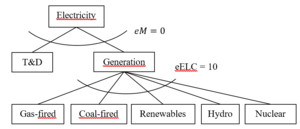
In later studies that focus on the energy sector, we employ a more elaborated structure for the power generation sector. The calibration of the power generation sector is based on the GTAP9-Power database, which is an electricity-detailed extension of Version 9 of the GTAP database (Aguiar et al., 2016; Peters, 2016). The GTAP9-Power database depicts the global economy in 2011 and provides data on 140 regions and 68 commodities. In the GRACE model, the power generation sector is divided into the five sub-sectors gas-fired plants, coal-fired plants, nuclear power, hydropower and renewables (see Figure 2.5 and 2.6a, b).
The power generation sector consists of generation, and transmission and distribution (T&D). Transmission and distribution are represented by a service sector, which is consumed in a fixed proportion relative to power generation, as described by a Leontief function (Peters, 2016b). Following many other CGE-based studies (e.g., Peters, 2016b; Sue Wing, 2008; Wing, 2006), we assume imperfect substitutability among technologies to depict market inertias associated with switching from one technology to another. Hence, a stricter climate policy will lead to substitution towards less carbon intensive technologies, without ending up with corner solutions. The choice of elasticity is subject to a compromise between a high elasticity to reflect the homogeneity of the output, and a low elasticity to reflect the incompleteness in switches between technologies.
Following Paltsev et al. (2005), we incorporate a technology-specific factor on the supply side of power generation from renewables, nuclear power, and hydro power. This can be interpreted as a natural resource constraint. The specific factor is assumed substitutable with the value added, meaning that we calibrate the substitution elasticity to achieve an assumed price elasticity of supply. There are only a few empirical estimates of the price elasticity of the supply of renewable electricity generation. For example, Johnson (2011) estimated a value of 2.7 for the price elasticity pertaining to the supply of renewables in the USA. This value was used by Paltsev et al. (2005) and Rivers (2013). In our analysis, we use the same value for renewables, whereas for nuclear power and hydropower, we use a value of 1 for the price elasticity of supply.
3.2) Capital and labour markets - GRACE
Economic growth is driven by investments, population growth, technological change and the availability of natural resources. Labour force growth is exogenously determined in the model and calibrated based on some population projection (e.g., World Bank). In the reference scenario, the real Gross Domestic Product (GDP) is exogenous and calibrated based on some economic growth projection (e.g., World Bank or OECD) by making labour productivity endogenous, i.e., a labour-augmenting technical change. Alternatively, the economic growth in the reference scenario could be calibrated by making total factor productivity endogenous (i.e., labour and capital). In policy simulations, factor endowment is scaled by the calibrated parameters of factor productivity and real GDP is endogenously determined within the model. Following the MIT EPPA6 model , we assume an annual autonomous energy efficiency improvement of 1.0% for non-electric sectors and 0.3% for the electric sector.
3.3) Monetary instruments - GRACE
Currently the model describes the real economy without a monetary model and hence no monetary instruments are involved so far.
3.4) Trade - GRACE
Total domestic output is distributed between export and domestic markets. In the core version of the GRACE model, domestic and export supplies are treated as perfect substitutes in production. In contrast, imported and domestically produced commodities are assumed imperfect substitutes. Following the Armington approach, we use a CES function to depict imperfect substitutability between imports and domestically produced goods, so that domestic and imported goods comprise the so-called Armington aggregate. In a two-level Armington aggregate, the first level depicts substitution in imports between regions, and the second level describes substitution between imported and domestically produced commodities. The Armington elasticities of substitution are obtained from the MIT EPPA model. Furthermore, importing countries pay a price premium to the international transport sector. This price premium is determined by a fixed transport factor derived from the base year data. The supply of international transport services is depicted by a Cobb-Douglas aggregate of the service good from the individual regions. The Armington aggregate is then distributed between private, public, investment, and intermediate consumption.
3.5) Technological change - GRACE
Technological change of energy and other production activities is generally exogenous in GRACE. In a reference scenario, technological change is calibrated to a given future pathway. In other scenarios, technological change is generallly the same as the reference scenarios without specific reasons.
4) Energy - GRACE
GRACE describes supply and demand of five energy carriers: coal, crude oil, gas, refined oil, and electricity. Depending on data availability, the electricity generation is further divided into generation technologies including coal-fueled, oil-fueled, gas-fueled, nuclear, hydro, wind, solar, and other renewable technologies. The supply and demand is simulated by nested CES functions.
4.1) Energy resource endowments - GRACE
Energy resource endowments are generally exogenous in GRACE. Depending on research questions, the endowments can be updated over time based on results from other energy models such as the energy model used by the International Energy Agency.
4.1.1) Fossil energy resources - GRACE
Fossil energy resources include resources for coal, oil, and gas, which are generally exogenous in GRACE. In some cases, the endowments can be updated over time based on results from other models.
4.1.2) Uranium and other fissile resources - GRACE
This is not considered in GRACE.
4.1.3) Bioenergy - GRACE
In GRACE, bioenergy can be generated from agriculture and forestry, and used to generate electricity.
4.1.4) Non-biomass renewables - GRACE
Non-biomass renewables in GRACE include hydro, nuclear, wind, and solar to generate electricity. The endowments of these renewables are exogenous in GRACE.
4.2) Energy conversion - GRACE
In GRACE, crude oil is used to produce refined oil products and electricity is generated from coal, gas, oil, nuclear, hydro and renewables. For more details, see the section of Production system and representation of economic sectors.
4.2.1) Electricity - GRACE
The electricity sector consists of power generation and transmission and distribution. Transmission and distribution are represented by a service sector. Imperfect substitutability among power generation technologies is assumed to depict market inertias associated with switching from one technology to another. GRACE simulates six technologies of power generation from coal, oil, gas, nuclear, hydro, and other renewables. Electricity is consumed by both industrial producers and households.
4.2.2) Heat - GRACE
GRACE does not simulate proudction and consumption of heat so far.
4.2.3) Gaseous fuels - GRACE
GRACE simulates production and consumption of only one gaseous fuel, i.e., natural gas. The production of natural gas is modeled as a nested CES function of intermediate inputs and primary factors. It can be used by industries, electricity generation, and households.
4.2.4) Liquid fuels - GRACE
GRACE simulates production and consumption of two liquid fuels, i.e., crude oil and refined oil. Their production is simulated as nested CES functions of intermediate inputs and primary factors. The liquid fuels can be used by industries, electricity generation, and households.
4.2.5) Solid fuels - GRACE
Solid fuels include coal and part of renewables. The coal production is modeled as a nested CES function of intermediate inputs and primary factors. Coal can be used by industries, electricity generation and households. Renewables are used for electricity generation.
4.2.6) Grid, pipelines and other infrastructure - GRACE
Grid is modeled as one part of electricity transmission and distribution. Services provided by pipelines for liquid and gaseous fuels are modeled as one part of the production of respective fuels. Other productive infrastructure is one part of capital assets in respective fuel production sectors.
4.3) Energy end-use - GRACE
Energy end-users in GRACE includes industrial producers and households, who consume coal, oil, gas, and electricity to produce goods for industries and satisfy consumption demand of households.
More details have been described in the section of Production system and representation of economic sectors.
4.3.1) Transport - GRACE
GRACE distinguish domestic and international transport.
Domestic transport in a region is divided into air, sea, and other transport activities, modeled as nested CES functions of energy use and other inputs.
Importing countries pay a price premium to the international transport sector. This price premium is determined by a fixed transport factor derived from the base year data. The supply of international transport services is depicted by a Cobb-Douglas aggregate of the service good from the individual regions. The Armington aggregate is then distributed between private, public, investment, and intermediate consumption.
4.3.2) Residential and commercial sectors - GRACE
GRACE simulates consumption of one residential sector - private households. The residential sector consumes coal, oil, gas and electricity as well as other consumption goods, following a combination of a nested CES function. Commercial activities are included in the activities of the only sector of services, which use coal, oil, gas and electricity as well as other inputs, following a combination of a nested CES function.
4.3.3) Industrial sector - GRACE
Industrial sector uses coal, oil, gas and electricity as well as other consumption goods, following a combination of a nested CES function.
4.3.4) Other end-use - GRACE
GRACE does not consider other end-use of energy goods so far.
4.4) Energy demand - GRACE
Energy demand is generally simulated as one group of inputs to energy consumers, who make a trade-off between energy use and other goods based on a behavior simulated by nested CES functions.
4.5) Technological change in energy - GRACE
Technological change in energy is exogenous. It is generally calibrated to obtain energy consumption and production in a given pathway of the future in a reference scenario. In alternative scenarios, the technological change in energy is assumed the same as the reference scenario without specific reasons.
5) Land-use - GRACE
Land use is one part of natural resources in GRACE. It is assumed exogenously given for each production sector based on available data. However, its productivity may vary depending on climate change impacts on agriculture, forestry, and fishery.
5.1) Agriculture - GRACE
Generally GRACE simulates only one sector of agriculture. In some cases focusing on agriculture, GRACE has divided the sector into four sub-sectors of wheat, rice, maize, and other agriculture (Wei et al. 2019). More details are available at the section of Production system and representation of economic sectors.
5.2) Forestry - GRACE
Generally GRACE simulates only one sector of agriculture. In some cases focusing on forestry, GRACE has included a specific module of forestry production (Aaheim et al. 2018). More details are available at the section of Production system and representation of economic sectors.
5.3) Land-use change - GRACE
Land use is one part of natural resources in GRACE. It is assumed exogenously given for each production sector based on available data. However, its productivity may vary depending on climate change impacts on agriculture, forestry, and fishery.
5.4) Bioenergy land-use - GRACE
So far, GRACE does not consider bioenergy land-use explicitly as bioenergy is not included in the model.
5.5) Other land-use - GRACE
GRACE does not consider other land-use so far.
5.6) Agricultural demand - GRACE
Agricultural products are used by industrial producers and households, generally as an input to nested CES functions. More details are available at the section of Production system and representation of economic sectors.
5.7) Technological change in land-use - GRACE
Generally no technological change is assumed in land-use by GRACE although it may be changed over time based on exogenous future pathways.
6) Emissions - GRACE
The GRACE model is suitable for analysing different mitigation policies since it can depict many policy instruments, such as carbon taxes and emissions permits. The base year CO2 emissions are provided by the GTAP database. Emissions permits are modelled as fixed-factor inputs (i.e., via a Leontief function). The latest version of the model also includes non-CO2 GHG emissions, such as methane (CH4), nitrous oxide (N2O), fluorinated gases (FGAS), which are provided by the GTAP database.
6.1) GHGs - GRACE
In GRACE, GHGs include CO2, methane (CH4), nitrous oxide (N2O), fluorinated gases (FGAS). In some cases, FGAS is further divided into HFC134a, HFC23, CF4, C2F6, C3F8, and C4F8 (Glomsrød et al. 2016). The emissions are modeled by assuming exogenous emission factors linked to energy use, natural resource use, and/or industrial production output.
6.2) Pollutants and non-GHG forcing agents - GRACE
It is possible to include non-GHG pollutants in GRACE although it is not the case in the core version. For example, a study (Glomsrød et al. 2016) has included air pollutants of aerosols and aerosol precursors (black carbon (BC), organic carbon (OC), sulfur dioxide (SO2), ammonia (NH3)), and ozone precursors (NOx, NMVOC, CO).
6.3) Carbon dioxide removal (CDR) options - GRACE
CDR options can added to GRACE although currently not considered in the model.
7) Climate - GRACE
It is possible to include a simple climate module in GRACE although currently it is not in place. At the moment, GRACE generates greenhouse gas emissions as inputs to simple or large climate models and the climate variables generated from climate models can be used as inputs to GRACE to disturb external environment of the global economic system. The soft-link to climate models enable GRACE to analyze the interactions between economic activities and climate change. For example, we can analyze climate and energy policy effect on global temperature and economic impact of climate change.
7.1) Modelling of climate indicators - GRACE
Climate indicators such as temperature and precipitation are introduced into GRACE as exogenous variables to disturb economics activities. The climate indicators are generally directly taken from results of other climate models. More about the impact functions are referred to Aaheim et al. (2012) and Aaheim et al. (2016).
7.2) Climate damages, temperature changes - GRACE
It is possible to include a simple climate module in GRACE although currently it is not in place. At the moment, GRACE generates greenhouse gas emissions as inputs to simple or large climate models and the climate variables generated from climate models can be used as inputs to GRACE to disturb external environment of the global economic system. The soft-link to climate models enable GRACE to analyze the interactions between economic activities and climate change. For example, we can analyze climate and energy policy effect on global temperature and economic impact of climate change.
8) Non-climate sustainability dimension - GRACE
GRACE describes the global and regional economy by region and sector. Hence, any sustainability issues related to the economy can potentially be analyzed by GRACE. For example, the United Nations Sustainable Development Goals (UN SDGs) on poverty, hunger, health and well-being, economic growth, consumption, production, and economic aspect of education and gender equality, water, energy, industry, inequalities, cities and communities.
8.1) Air pollution and health - GRACE
Generally GRACE does not consider the relations between air pollution and health. Potentially, the health impact of air pollution can be explicitly simuated by an additional module in GRACE.
8.2) Water - GRACE
Generally GRACE simulates production and consumption of only one water sector. More details are available at the section of Production system and representation of economic sectors.
8.3) Other materials - GRACE
GRACE describes the global and regional economy by region and sector. Hence, any sustainability issues related to the economy can potentially be analyzed by GRACE. For example, the United Nations Sustainable Development Goals (UN SDGs) on poverty, hunger, health and well-being, economic growth, consumption, production, and economic aspect of education and gender equality, water, energy, industry, inequalities, cities and communities.
8.4) Other sustainability dimensions - GRACE
GRACE describes the global and regional economy by region and sector. Hence, any sustainability issues related to the economy can potentially be analyzed by GRACE. For example, the United Nations Sustainable Development Goals (UN SDGs) on poverty, hunger, health and well-being, economic growth, consumption, production, and economic aspect of education and gender equality, water, energy, industry, inequalities, cities and communities.
9) Appendices - GRACE
9.1) Mathematical model description - GRACE
Mathematical model description of GRACE is available at http://hdl.handle.net/11250/2480843
9.2) Data - GRACE
GTAP database at https://www.gtap.agecon.purdue.edu/databases World population data at https://population.un.org/wpp/
10) References - GRACE
AGUIAR, A., CHEPELIEV, M., CORONG, E. L., MCDOUGALL, R. & VAN DER MENSBRUGGHE, D. 2019. The GTAP Data Base: Version 10. Journal of Global Economic Analysis, 4, 1-27.
CARATTINI, S., KALLBEKKEN, S. & ORLOV, A. 2019. How to win public support for a global carbon tax. Nature, 565, 289–291.
CRIPPA, M., GUIZZARDI, D., MUNTEAN, M., SCHAAF, E., DENTENER, F., VAN AARDENNE, J. A., MONNI, S., DOERING, U., OLIVIER, J. G. J., PAGLIARI, V. & JANSSENS-MAENHOUT, G. 2018. Gridded Emissions of Air Pollutants for the period 1970-2012 within EDGAR v4.3.2. Earth Syst. Sci. Data Discuss., 2018, 1-40.
ESKELAND, G. S., RIVE, N. A. & MIDEKSA, T. K. 2012. Europe’s climate goals and the electricity sector. Energy Policy, 41, 200–211.
GLOMSRØD, S. & WEI, T. 2016. The effects of energy efficiency improvement in China with global interaction. AIMS Energy, 4, 37-51.
GLOMSRØD, S. & WEI, T. 2018. Business as unusual: The implications of fossil divestment and green bonds for financial flows, economic growth and energy market. Energy for Sustainable Development, 44, 1-10.
GLOMSRØD, S., WEI, T. & ALFSEN, K. 2013. Pledges for climate mitigation: the effects of the Copenhagen accord on CO2 emissions and mitigation costs. Mitigation and Adaptation Strategies for Global Change, 18, 619–636.
GLOMSRØD, S., WEI, T., MIDEKSA, T. & SAMSET, B. 2015. Energy market impacts of nuclear power phase-out policies. Mitigation and Adaptation Strategies for Global Change, 20, 1511-1527.
GLOMSRØD, S., WEI, T., AAMAAS, B., LUND, M. T. & SAMSET, B. H. 2016. A warmer policy for a colder climate: Can China both reduce poverty and cap carbon emissions? Science of The Total Environment, 568, 236-244.
LIU, Y. & WEI, T. 2016. Linking the emissions trading schemes of Europe and China - Combining climate and energy policy instruments. Mitigation and Adaptation Strategies for Global Change, 21, 135-151.
ORLOV, A. 2017. Distributional effects of higher natural gas prices in Russia. Energy Policy, 109, 590-600.
ORLOV, A., SILLMANN, J., AUNAN, K., KJELLSTROM, T. & AAHEIM, A. 2020. Economic costs of heat-induced reductions in worker productivity due to global warming. Global Environmental Change, 63, 102087.
ORLOV, A. & AAHEIM, A. 2017. Economy-wide effects of international and Russia's climate policies. Energy Economics, 68, 466-477.
RIVE, N. 2010. Climate policy in Western Europe and avoided costs of air pollution control. Economic Modelling, 27, 103-115.
RIVE, N. & MIDEKSA, T. K. 2009. Disaggregating the Electricity Sector in the GRACE Model. Report. Oslo, Norway: CICERO.
RIVE, N. & RÜBBELKE, D. G. 2010. International environmental policy and poverty alleviation. Review of World Economics, 146, 515-543.
ROSON, R. & SARTORI, M. 2016. Estimation of Climate Change Damage Functions for 140 Regions in the GTAP 9 Data Base. Journal of Global Economic Analysis, 1, 78-115.
RYPDAL, K., RIVE, N., ÅSTRÖM, S., KARVOSENOJA, N., AUNAN, K., BAK, J. L., KUPIAINEN, K. & KUKKONEN, J. 2007. Nordic air quality co-benefits from European post-2012 climate policies. Energy Policy, 35, 6309–6322.
UNDERDAL, A. & WEI, T. 2015. Distributive fairness: A mutual recognition approach. Environmental Science & Policy, 51, 35-44.
WEI, T. 2019. The global CGE model (GRACE) at CICERO [Online]. Available: http://folk.uio.no/taoyuaw/grace.htm [Accessed 30 Mar. 2019].
WEI, T., GLOMSRØD, S. & ZHANG, T. 2017. Extreme weather, food security and the capacity to adapt – the case of crops in China. Food Security, 9, 523-535.
WEI, T. & LIU, Y. 2017. Estimation of global rebound effect caused by energy efficiency improvement. Energy Economics, 66, 27-34.
WEI, T., ZHU, Q. & GLOMSRØD, S. 2018a. Ageing Impact on the Economy and Emissions in China: A Global Computable General Equilibrium Analysis. Energies, 11, 817.
WEI, T., ZHU, Q. & GLOMSRØD, S. 2018b. How Will Demographic Characteristics of the Labor Force Matter for the Global Economy and Carbon Dioxide Emissions? Ecological Economics, 147, 197-207.
WEI, T. Y., ZHANG, T. Y., CUI, X. F., GLOMSROD, S. & LIU, Y. 2019. Potential Influence of Climate Change on Grain Self-Sufficiency at the Country Level Considering Adaptation Measures. Earths Future.
WU, Z. 2004. Wage curve for urban China: a panel data approach. Applied Economics Letters, 11, 425-428.
ZHU, Q. & WEI, T. 2017. Implications of population aging for labor supply and economic growth in China: A CGE Analysis. Population Research, 41, 8-21.
AAHEIM, A., AMUNDSEN, H., DOKKEN, T. & WEI, T. 2012. Impacts and adaptation to climate change in European economies. Global Environmental Change-Human and Policy Dimensions, 22, 959–968.
AAHEIM, A., GOPALAKRISHNAN, R., CHATURVEDI, R., RAVINDRANATH, N., SAGADEVAN, A., SHARMA, N. & WEI, T. 2011. A macroeconomic analysis of adaptation to climate change impacts on forests in India. Mitigation and Adaptation Strategies for Global Change, 16, 229-245.
AAHEIM, A., ORLOV, A., CHATURVEDI, R. K., JOSHI, P., SAGADEVAN, A. & RAVINDRANATH, N. H. 2018a. Lost benefits and carbon uptake by protection of Indian plantations. Mitigation and Adaptation Strategies for Global Change, 23, 485-505.
AAHEIM, A., ORLOV, A., WEI, T. & GLOMSRØD, S. 2018b. GRACE model and applications. Report. Oslo, Norway: CICERO.
AAHEIM, A. & RIVE, N. 2005. A Model for Global Responses to Anthropogenic Changes in the Environment (GRACE). Report. Oslo, Norway: CICERO.
AAHEIM, A., ROMSTAD, B., WEI, T., KRISTJÁNSSON, J. E., MURI, H., NIEMEIER, U. & SCHMIDT, H. 2015. An economic evaluation of solar radiation management. Science of The Total Environment, 532, 61-69.
AAHEIM, A., WEI, T. & ROMSTAD, B. 2016. Conflicts of economic interests by limiting global warming to +3 °C. Mitigation and Adaptation Strategies for Global Change, 22, 1131-1148.
Note: Flexible based on the latest GTAP database.