Snapshot of - TIAM-UCL
Archive of TIAM-UCL, version: 1.0
Reference card - TIAM-UCL
The reference card is a clearly defined description of model features. The numerous options have been organized into a limited amount of default and model specific (non default) options. In addition some features are described by a short clarifying text.
Legend:
- not implemented
- implemented
- implemented (not default option)
About
Name and version
TIAM-UCL 1.0
Institution
University College London (UCL), UK, https://www.ucl.ac.uk.
Documentation
TIAM-UCL documentation consists of a referencecard and detailed model documentation
Process state
published
Model scope and methods
Model documentation: Model scope and methods - TIAM-UCL
Model type
- Integrated assessment model
- Energy system model
- CGE
- CBA-integrated assessment model
Geographical scope
- Global
- Regional
Objective
TIAM-UCL (TIMES Integrated Assessment Model) uses the TIMES modelling platform, which is a successor of the MARKAL platform. The markal/times modelling concept was originally intended to analyse energy systems at a regional or global level and has evolved to also describe greenhouse gas emissions. Scenario based simulations maximize the total discounted sum of consumer and supplier surplus over the model horizon, while taking into account the constraints (e.g. energy demand to be fulfilled, availability of energy resources etc).
Solution concept
- Partial equilibrium (price elastic demand)
- Partial equilibrium (fixed demand)
- General equilibrium (closed economy)
Solution horizon
- Recursive dynamic (myopic)
- Intertemporal optimization (foresight)
Solution method
- Simulation
- Optimization
- Linear optimisation
Anticipation
Perfect Foresight (Stochastic and myopic runs are also possible)
Temporal dimension
Base year:2005, time steps:5 years up to 2050 and 10 years beyond (changeable), horizon: 95 years (2005-2100)
Spatial dimension
Number of regions:16
- Africa
- Australia
- Canada
- Central and South America
- China
- Eastern Europe
- Former Soviet Union
- India
- Japan
- Mexico
- Middle East
- Other Developing Asia
- South Korea
- United Kingdom
- United States of Amercia
- Western Europe
Note: UK split as separate region compared to the ETSAP-TIAM model
Time discounting type
- Discount rate exogenous
- Discount rate endogenous
Policies
- Emission tax
- Emission pricing
- Cap and trade
- Fuel taxes
- Fuel subsidies
- Feed-in-tariff
- Portfolio standard
- Capacity targets
- Emission standards
- Energy efficiency standards
- Agricultural producer subsidies
- Agricultural consumer subsidies
- Land protection
- Pricing carbon stocks
Socio-economic drivers
Model documentation: Socio-economic drivers - TIAM-UCL
Population
- Yes (exogenous)
- Yes (endogenous)
Population age structure
- Yes (exogenous)
- Yes (endogenous)
Education level
- Yes (exogenous)
- Yes (endogenous)
Urbanization rate
- Yes (exogenous)
- Yes (endogenous)
GDP
- Yes (exogenous)
- Yes (endogenous)
Income distribution
- Yes (exogenous)
- Yes (endogenous)
Employment rate
- Yes (exogenous)
- Yes (endogenous)
Labor productivity
- Yes (exogenous)
- Yes (endogenous)
Total factor productivity
- Yes (exogenous)
- Yes (endogenous)
Autonomous energy efficiency improvements
- Yes (exogenous)
- Yes (endogenous)
Macro-economy
Model documentation: Macro-economy - TIAM-UCL
Economic sector
Industry
- Yes (physical)
- Yes (economic)
- Yes (physical & economic)
Energy
- Yes (physical)
- Yes (economic)
- Yes (physical & economic)
Transportation
- Yes (physical)
- Yes (economic)
- Yes (physical & economic)
Residential and commercial
- Yes (physical)
- Yes (economic)
- Yes (physical & economic)
Agriculture
- Yes (physical)
- Yes (economic)
- Yes (physical & economic)
Forestry
- Yes (physical)
- Yes (economic)
- Yes (physical & economic)
Other economic sector
Note: Link with MACRO Stand-Alone (module which represents all other economic sectors) available to represent rest of the economy
Macro-economy
Trade
- Coal
- Oil
- Gas
- Uranium
- Electricity
- Bioenergy crops
- Food crops
- Capital
- Emissions permits
- Non-energy goods
- Diesel
- LNG
- Gasoline
- Heavy fuel oil
- Natural gas liquids
- Naphtha
Cost measures
- GDP loss
- Welfare loss
- Consumption loss
- Area under MAC
- Energy system cost mark-up
Categorization by group
- Income
- Urban - rural
- Technology adoption
- Age
- Gender
- Education level
- Household size
Institutional and political factors
- Early retirement of capital allowed
- Interest rates differentiated by country/region
- Regional risk factors included
- Technology costs differentiated by country/region
- Technological change differentiated by country/region
- Behavioural change differentiated by country/region
- Constraints on cross country financial transfers
Resource use
Coal
- Yes (fixed)
- Yes (supply curve)
- Yes (process model)
Conventional Oil
- Yes (fixed)
- Yes (supply curve)
- Yes (process model)
Unconventional Oil
- Yes (fixed)
- Yes (supply curve)
- Yes (process model)
Conventional Gas
- Yes (fixed)
- Yes (supply curve)
- Yes (process model)
Unconventional Gas
- Yes (fixed)
- Yes (supply curve)
- Yes (process model)
Uranium
- Yes (fixed)
- Yes (supply curve)
- Yes (process model)
Bioenergy
- Yes (fixed)
- Yes (supply curve)
- Yes (process model)
Water
- Yes (fixed)
- Yes (supply curve)
- Yes (process model)
Raw Materials
- Yes (fixed)
- Yes (supply curve)
- Yes (process model)
Land
- Yes (fixed)
- Yes (supply curve)
- Yes (process model)
Technological change
Energy conversion technologies
- No technological change
- Exogenous technological change
- Endogenous technological change
Energy End-use
- No technological change
- Exogenous technological change
- Endogenous technological change
Material Use
- No technological change
- Exogenous technological change
- Endogenous technological change
Agriculture (tc)
- No technological change
- Exogenous technological change
- Endogenous technological change
Energy
Model documentation: Energy - TIAM-UCL
Behaviour
Elastic demand mode available (includes exogenous elasticity of each energy demand with respect to their own price) Technology and region specific hurdle rates.
Energy technology substitution
Energy technology choice
- No discrete technology choices
- Logit choice model
- Production function
- Linear choice (lowest cost)
- Lowest cost with adjustment penalties
Energy technology substitutability
- Mostly high substitutability
- Mostly low substitutability
- Mixed high and low substitutability
Energy technology deployment
- Expansion and decline constraints
- System integration constraints
Energy
Electricity technologies
- Coal w/o CCS
- Coal w/ CCS
- Gas w/o CCS
- Gas w/ CCS
- Oil w/o CCS
- Oil w/ CCS
- Bioenergy w/o CCS
- Bioenergy w/ CCS
- Geothermal power
- Nuclear power
- Solar power
- Solar power-central PV
- Solar power-distributed PV
- Solar power-CSP
- Wind power
- Wind power-onshore
- Wind power-offshore
- Hydroelectric power
- Ocean power
Hydrogen production
- Coal to hydrogen w/o CCS
- Coal to hydrogen w/ CCS
- Natural gas to hydrogen w/o CCS
- Natural gas to hydrogen w/ CCS
- Oil to hydrogen w/o CCS
- Oil to hydrogen w/ CCS
- Biomass to hydrogen w/o CCS
- Biomass to hydrogen w/ CCS
- Nuclear thermochemical hydrogen
- Solar thermochemical hydrogen
- Electrolysis
Refined liquids
- Coal to liquids w/o CCS
- Coal to liquids w/ CCS
- Gas to liquids w/o CCS
- Gas to liquids w/ CCS
- Bioliquids w/o CCS
- Bioliquids w/ CCS
- Oil refining
Refined gases
- Coal to gas w/o CCS
- Coal to gas w/ CCS
- Oil to gas w/o CCS
- Oil to gas w/ CCS
- Biomass to gas w/o CCS
- Biomass to gas w/ CCS
Heat generation
- Coal heat
- Natural gas heat
- Oil heat
- Biomass heat
- Geothermal heat
- Solarthermal heat
- CHP (coupled heat and power)
Grid Infra Structure
Electricity
- Yes (aggregate)
- Yes (spatially explicit)
Gas
- Yes (aggregate)
- Yes (spatially explicit)
Heat
- Yes (aggregate)
- Yes (spatially explicit)
CO2
- Yes (aggregate)
- Yes (spatially explicit)
Hydrogen
- Yes (aggregate)
- Yes (spatially explicit)
Other grid and infrastructure
Note: No explicit modelling of grids, only a transmission cost and division to centralised/decentralised electricity generation technologies
Energy end-use technologies
Passenger transportation
- Passenger trains
- Buses
- Light Duty Vehicles (LDVs)
- Electric LDVs
- Hydrogen LDVs
- Hybrid LDVs
- Gasoline LDVs
- Diesel LDVs
- Passenger aircrafts
Freight transportation
- Freight trains
- Heavy duty vehicles
- Freight aircrafts
- Freight ships
Industry
- Steel production
- Aluminium production
- Cement production
- Petrochemical production
- Paper production
- Plastics production
- Pulp production
- Chemicals
- Iron and steel
- Pulp and paper
- Non metals
- Other Industries
- Non-ferrous metals
- Other non-energy
- Other non-specified
Residential and commercial
- Space heating
- Space cooling
- Cooking
- Refrigeration
- Washing
- Lighting
- Water heating
- Clothes drying
- Other electrical uses
- Other non-electrical uses
Note: Washing is disaggregated in clothes and dishes.
Land-use
Model documentation: Land-use - TIAM-UCL
Land cover
- Cropland
- Cropland irrigated
- Cropland food crops
- Cropland feed crops
- Cropland energy crops
- Forest
- Managed forest
- Natural forest
- Pasture
- Shrubland
- Built-up area
Agriculture and forestry demands
- Agriculture food
- Agriculture food crops
- Agriculture food livestock
- Agriculture feed
- Agriculture feed crops
- Agriculture feed livestock
- Agriculture non-food
- Agriculture non-food crops
- Agriculture non-food livestock
- Agriculture bioenergy
- Agriculture residues
- Forest industrial roundwood
- Forest fuelwood
- Forest residues
Agricultural commodities
- Wheat
- Rice
- Other coarse grains
- Oilseeds
- Sugar crops
- Ruminant meat
- Non-ruminant meat and eggs
- Dairy products
Emission, climate and impacts
Model documentation: Emissions - TIAM-UCL, Climate - TIAM-UCL, Non-climate sustainability dimension - TIAM-UCL
Greenhouse gases
- CO2 fossil fuels
- CO2 cement
- CO2 land use
- CH4 energy
- CH4 land use
- CH4 other
- N2O energy
- N2O land use
- N2O other
- CFCs
- HFCs
- SF6
- PFCs
Note: Some emissions are exogenous (eg: agriculture)
Pollutants
- CO energy
- CO land use
- CO other
- NOx energy
- NOx land use
- NOx other
- VOC energy
- VOC land use
- VOC other
- SO2 energy
- SO2 land use
- SO2 other
- BC energy
- BC land use
- BC other
- OC energy
- OC land use
- OC other
- NH3 energy
- NH3 land use
- NH3 other
Climate indicators
- Concentration: CO2
- Concentration: CH4
- Concentration: N2O
- Concentration: Kyoto gases
- Radiative forcing: CO2
- Radiative forcing: CH4
- Radiative forcing: N2O
- Radiative forcing: F-gases
- Radiative forcing: Kyoto gases
- Radiative forcing: aerosols
- Radiative forcing: land albedo
- Radiative forcing: AN3A
- Radiative forcing: total
- Temperature change
- Sea level rise
- Ocean acidification
Note: Climate damages available although not often modelled CO2 is from both energy and also land-use (and forestry) included in climate module. The non-CO2 forcing agents that are not explicitly tracked are represented in the climate module by an exogenously given additional forcing factor.
Carbon dioxide removal
- Bioenergy with CCS
- Reforestation
- Afforestation
- Soil carbon enhancement
- Direct air capture
- Enhanced weathering
Climate change impacts
- Agriculture
- Energy supply
- Energy demand
- Economic output
- Built capital
- Inequality
Co-Linkages
- Energy security: Fossil fuel imports & exports (region)
- Energy access: Household energy consumption
- Air pollution & health: Source-based aerosol emissions
- Air pollution & health: Health impacts of air Pollution
- Food access
- Water availability
- Biodiversity
Model Documentation - TIAM-UCL
TIAM-UCL is a global energy systems model that is usually run along with a climate module (calibrated to MAGICC) and an aggregated economic module (Macro Stand-Alone) in order to assess long-term energy decarbonisation scenarios and pathways.
The model is called the TIMES Integrated Assessment Model in UCL. TIMES is itself an acronym for ‘The Integrated MARKAL-EFOM System’.
The framework is akin to that of a long-term social planner with perfect foresight that acheives exogenous energy demands at lowest cost given detailed energy technology assumptions and specified constraints
1) Model scope and methods - TIAM-UCL
TIAM-UCL is a bottom-up, technology-rich cost optimisation integrated assessment model created to assess the energy system costs of global decarbonisation pathways in terms of the global temperature change and/or carbon budgets.
1.1) Model concept, solver and details - TIAM-UCL
The main building blocks of TIAM-UCL is a TIMES model which includes processes and commodities, which are connected by commodity flows in a network representation called a Reference Energy System (RES). The model dynamics are determined by the time horizon and resolution, the evolutionary development of supply and technologies, the growth of the demand for energy services, and policies (e.g., mitigation targets, renewable portfolio standards), complimented by various alternate scenarios.
<figure id="fig:myobject">
</figure>
In each region, the TIAM-UCL model describes the entire energy system by all essential current and future energy technologies from the primary energy supply over the processing, conversion, transport, distribution of energy carriers to the end-use sectors and the useful energy demands. These demands are linked to exogenous underlying drivers, like population growth or GDP development, via demand elasticities. Each region can trade one or more resources (fossil fuels and biomass) with other regions. Regional trade will depend on demand, supply (resource availability) and cost (resource and transportation cost) of the resources.
Base-year energy-service demands are exogenous and projected over 2005-2100 using drivers such as GDP, population, household, sector output etc. The base year (2005) final energy consumption is calibrated in the Base-Year templates module. Separate BY templates are available for each region for all end-use sectors, upstream, and the electricity generation sector. A representation of all existing technologies and resources are included in the Base-Year templates to determine the state of teh energy system in the intial period. Technologies available for the future years are modelled in a separate module called 'New Technologies'. Any region can access the technology module if it is cost effective to do so. Resource data such as cost, cumulative and annual availability of different resources are modelled in the 'Resource Module'. The world regions are linked through the trade of energy goods and CO2 via the trade module. There are separate modules available for hydrogen production, carbon sequestration, land-use CO2 emissions, N2O measures, CH4 measures, etc. Climate module calculates impacts of GHG emissions in the Atmosphere (CO2 concentration and temperature changes). Beside these modules, there are several scenario files which are used to apply different policies and constraints.
Further details on the TIAM model structure is available in Loulou and Labriet (2007).
The underlying data for the base year calibration in TIAM-UCL is the IEA Extended Energy Balances of OECD and non-OECD countries.
Software
TIAM is a whole energy system model covering from energy resources to conversion to infrastructure to end-use sectors.This is a linear programming model that minimises total discounted energy system cost in the standard version and maximises societal welfare (total surplus) in the elastic demand version to compute a partial equilibrium. Linear programming is formulated in the GAMS (General Algebraic Modelling System) language and solved via powerful linear programming optimisers (CPLEX, XPRESS or others).
VEDA Front-End (VEDA_FE) is one of the two interfaces available for the TIMES model. It is used to formulate the TIAM-UCL model database that lay down the basic structure of the model and hold fundamental data and assumptions for processes (technologies) and commodities. VEDA is a set of tools geared to facilitate the creation, maintenance, browsing, and modification of the large data bases required by complex mathematical and economic models. Data and assumptions are fed into VEDA_FE that provides input to the TIMES code. VEDA_FE accepts input from a variety of Excel files with different (flexible) structures that are tailored to work efficiently with data intensive models. The model is sent from VEDA_FE to GAMS where it is run. The results are then loaded into another interface, VEDA Back-End (VEDA_BE), where they can be manipulated and interpreted as necessary.
Modelling to Generate Alternatives
A critical challenge when working with global energy-environment-economy (E3) models is appropriately exploring the large uncertainties inherent in the modelling procedure. Without careful elucidation, analysts and policy makers alike can be misled by the precision of the model output and lured into a false sense of security at the certainty of the implied energy system transition(s). Broadly speaking, uncertainty in E3 models can be separated into input parameter uncertainty and structural uncertainty. Our focus here is on the latter, which stems from the model not fully capturing the complexity of the system it is trying to represent because, for example, it has necessarily simplified equations, a finite resolution, etc. Over the course of the ADVANCE project we have developed a technique to investigate a key element of structural uncertainty within TIAM-UCL. We have used the approach of modelling to generate alternatives to relax the cost optimality assumption that underpins the model and reformulated its objective function to explore this near optimal solution space. Our technique seeks to identify energy system transition pathways that are as diverse as possible within this near least cost space and as such assess the impact of minor, realistic deviations from cost optimal decision making.
1.3) Temporal dimension - TIAM-UCL
The model base year is 2005 with data taken from IEA Energy Balances.
The model time horizon is 95 years (2005-2100) with 5 year time steps up to 2070 and with 10 year time steps beyond. Each year is divided to six time slices + an additional peaking constraint.
Demand fractions (see Table 1.2) determine the fraction of service demand to be met during a specific period of the day in a given season (or timeslice).
The temporal resolution is determined by three seasons, summer, winter and intermediate. Each of the seasons accounts for a third of the whole year or 4 month. These timeslices are again split into night and day, where day represents 16 hours and night 8 hours (Table 1-2).
Therefore there a six timeslice possibilities of:
- summer-day,
- summer-night,
- intermediary day,
- intermediary-night,
- winter-day,
- winter-night
Table 1.2: Fraction of energy-service demands
| Time slice | Month share | Day share | Fraction |
| ID | 0.333 (4 months) | 0.666 (16 hours) | 0.223 |
| IN | 0.333 (8 hours) | 0.111 | |
| SD | 0.333 | 0.666 | 0.223 |
| SN | 0.333 | 0.111 | |
| WD | 0.333 | 0.666 | 0.221 |
| WN | 0.333 | 0.111 |
The model is generally run with perfect foresight but can be run as myopic or stochastic though this is generally not the case.
1.4) Spatial dimension - TIAM-UCL
TIAM-UCL is a global model with 16 regions listed in the table below, each of which has their own energy system.
The TIAM-UCL model has been developed at UCL since 2010 and differs from the ETSAP-TIAM model in two ways: the first is breaking out the UK from the 15 region ETSAP-TIAM model; the second is enhancing TIAM-UCL by revising/adding new drivers and resources for all regions and adding new features.
In order to break out the UK from Western Europe (WEU) region, separate Base-Year templates were created for end-use sectors, upstream and power sectors for the UK and calibrated final energy consumption to the actual base year data 2005 for the UK and the WEU regions. The underlying data for the base year calibration in TIAM-UCL is the IEA Extended Energy Balances of OECD and non-OECD countries. This data can be accessed through the online portal https://www.ukdataservice.ac.uk/ in the UK. A database of the IEA Extended Energy Balances has been developed to import the IEA data into the data tables on the base year templates in the TIAM-UCL with a software application which allows easy aggregation of country data into regions. Energy services demands for different end-use sectors and drivers of projections of demands during the model period 2005-2100 were created for the UK region. Besides the calibration of resource and trade modules of the UK and the WEU regions, all other scenario files were also updated and calibrated.
Once the 16 region TIAM-UCL had been successfully calibrated, the model was enhanced through technical improvements such as adding new drivers, new resources, climate change policies (cap-and-trade, carbon tax), supply resource cost curves etc. Development of the database of the IEA Extended Energy Balances helped to recalibrate all 16 regions in the TIAM model to the IEA primary energy production/consumption, final consumption and electricity generation (and heat) data.
Table 1.1: Regions in TIAM-UCL
| Region | Countries |
| Africa (AFR) | Algeria, Angola, Benin, Cameroon, Congo, Congo Republic, Egypt, Ethiopia, Gabon, Ghana, Ivory Coast, Kenya, Libya, Morocco, Mozambique, Nigeria, Other Africa, Senegal, South Africa, Sudan, Tanzania, Tunisia, Zambia, Zimbabwe |
| Australia (AUS) | Australia and New Zealand |
| Canada (CAN) | Canada |
| Central and South America (CSA) | Argentina, Bolivia, Brazil, Chile, Colombia, Costa Rica, Cuba, Dominican Republic, Ecuador, El Salvador, Guatemala, Haiti, Honduras, Jamaica, Netherlands Antilles, Nicaragua, Other Latin America, Panama, Paraguay, Peru, Trinidad-Tobago, Uruguay, Venezuela |
| China (CHI) | China |
| Eastern Europe (EEU) | Albania, Bosnia-Herzegovina, Bulgaria, Croatia, Czech Republic, Hungary, Macedonia, Poland, Romania, Slovakia, Slovenia, Yugoslavia |
| Former Soviet Union (FSU) | Armenia, Azerbaijan, Belarus, Estonia, Georgia, Kazakhstan, Kyrgyzstan, Latvia, Lithuania, Moldova, Russia, Tajikistan, Turkmenistan, Ukraine, Uzbekistan |
| India (IND) | India |
| Japan (JAP) | Japan |
| Mexico (MEX) | Mexico |
| Middle-east (MEA) | Bahrain, Cyprus, Iran, Iraq, Israel, Jordan, Kuwait, Lebanon, Oman, Qatar, Saudi Arabia, Syria, Turkey, United Arab Emirates, Yemen |
| Other Developing Asia (ODA) | Bangladesh, Brunei, Chinese Taipei, Indonesia, North Korea, Malaysia, Myanmar, Nepal, Other Asia, Pakistan, Philippines, Singapore, Sri Lanka, Thailand, Vietnam |
| South Korea (SKO) | South Korea |
| United Kingdom (UK) | United Kingdom |
| USA (USA) | United States of America |
| Western Europe (WEU) | Austria, Belgium, Denmark, Finland, France, Germany, Gibraltar, Greece, Greenland, Iceland, Ireland, Italy, Luxembourg, Malta, Netherlands, Norway, Portugal, Spain, Sweden, Switzerland |
1.5) Policy - TIAM-UCL
A variety of energy and climate policies can be implemented, depending on the approach, usually by creating specific scenario files to incorporate the policy elements.
A number of general or specific policy choices can be modelled including:
- Emissions taxes,
- permit trading,
- specific technology subsidies
- Technology and/or resource constraints
- Technology and/or resource targets
2) Socio-economic drivers - TIAM-UCL
There are 42 energy-service demands for the five different end-use sectors in TIAM-UCL.
A driver is allocated to each energy service demand to project demand for future years throughout the model horizon (2005 to 2100). The driver is linked to the energy-service demand by a constant and an elasticity. Demand drivers include population, GDP, number of households, GDP per capita, GDP per household and agricultural, service and industrial drivers.
Assumptions on the development of drivers are based on several sources, which are explained in the following subsections. Assumptions on demand drivers have been substantially updated from the ESTAP-TIAM model.
2.1) Population - TIAM-UCL
Population
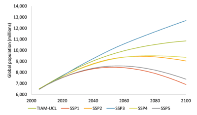
Population figures up to 2050 are based on UN estimations (UN, 2009). It is assumed that world population will increase from 6.7 billion people in 2005 to 9.3 billion people in 2050, reach the peak in 2090 with 9.8 billion and then decline slightly.
The biggest population increase over the 21st century is expected to happen in Africa, India, Other Developing Asia and the Middle East .
Under the given assumptions China, Eastern Europe, Former Soviet Union, Japan, Mexico, South Korea and Western Europe experience negative population growth rates in the second half of the 21st century.
Especially for South Korea and Japan, it is assumed that the population will shrink significantly over the course of the 21st century.
We are also able to run the various Shared Socio-economic (SSP) pathway scenarios nakicenovic2014a in TIAM-UCL. The standard TIAM-UCL population assumption is around halfway between SSP3 and SSP2 for population.
<figure id="fig:Population SSPs">
 </figure>
Households
The number of households is based on population estimates and occupancy rate. There exists no database for the occupancy rate for each region in the TIAM-UCL model. Therefore, the numbers in this section rely on national statistics. There are forecasts for the average household occupancy for some countries for the near future (up to 2030) from which it is possible estimate the number of households (given assumptions on population). For the longer term, it is assumed that the occupancy rate will increase in line with historic data to 1.7 to 3 persons per household, depending on the region. The reason for this range is the difference in current average persons per household, e.g. in 2005 the average Indian household consisted of 5.3 persons, while the average Western European household consisted of 2.1 persons per household.
Given these assumptions, the total number of households globally increases from 1.9 billion in 2005 to 3.4 billion in 2050 to 5.1 billion in 2100.
In order to simplify the data needed for the calculation, characteristic countries have been chosen for regions that consist of more than two countries. Those are South Africa for Africa, Brazil for Central and South America, Poland for Eastern Europe, Russia for Former Soviet Union, Iran for Middle East, Indonesia for Other Developing Asia and Germany for Western Europe.
2.2) Economic activity - TIAM-UCL
GDP
Estimations of future economic growth are much more uncertain than future population growth. Few studies exist that forecast GDP up to 2100 and so unlike population assumptions, GDP figures in TIAM-UCL are not based on a single source. Economic growth rates have been compared to assumptions made for scenarios in the 4th assessment report of the IPCC (Tsuneyuki 1999) and Clarke et al. (2007). Global GDP is assumed to grow from $50 trillion in 2010 to $155 trillion in 2050 and $350 trillion in 2100 (all GDP are in 2005 US$). Current figures for 2010 have been taken from the IMF (2009).
Figures for future economic growth are based on an approximate assumption of economic convergence between regions (see Figure 3 5), i.e. that low income regions grow faster compared to high income regions. The figure shows this convergence of per capita income among world regions. The GDP per person is calculated as the ratio of GDP and population. The economic convergence is a central point in the assumptions on socio-economic drivers. The effect becomes clear when one compares the GDP per head in different regions. In 2005 India is the poorest region with a GDP per head of 10% of the world average and the USA is the richest region with 600% of the world average. In 2100 this picture changes with India having a GDP per head that has now grown to 55% of the world average and the USA being the richest country with 350% of the world average.
GDP growth rates are expected to decline over the course of the 21st century, while they remain higher for developing countries than for developed countries. Owing to the shrinking population, the growth rates for South Korea and Japan are very low and turn negative at the end of the 21st century. Growth rates for Western Europe, the UK and the United States are assumed to drop from an average of 2.2% to 1.3% p.a. in 2050. The only region that is expected to increase GDP growth rates over the first decades is Africa based on a growing population and its current low income levels. Global economic growth is approximately in the mid-range of the growth in the SSP scenarios
<figure id="fig:GDP per capita">
 </figure>
Sectoral drivers
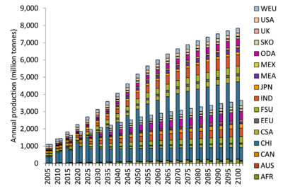
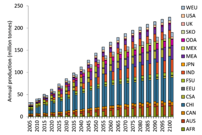
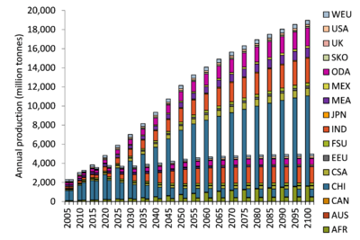
The industrial, services and agricultural sectors have different growth drivers from all other sectors i.e. they are not directly related to growth in GDP and a decoupling factor. There are a number of reasons for this, but key is that there is expected to be a decoupling of growth in, for example, production of steel and growth in GDP that is cannot be trivially estimated by a single decoupling factor. Additionally, the industrial service demands can be interpreted as represent the production of physical quantities e.g. tonnes of steel, tonnes of aluminium etc. Projections of future production are provided by various sources, who look in detail at the array of factors that affect production and consumption levels on regional basis. These sources therefore likely provide more robust estimates of future production while also providing a more tangible projection of what is being estimated.
The projections of steel, aluminium and cement, paper and chemicals production globally used in TIAM-UCL are provided in the Figures below. These figures also shows how these compare with the projections used in ETSAP-TIAM. These quantities have been estimated using the regional per-capita consumption and productions projections from IEA up to 2050 ensuring that these balance on a global level). A single provider was used for this estimation to ensure consistency across the different metallic and non-metallic sectors. Consumption from 2050 to 2100 was then based on historical trends in per-capita consumption from 2000 to 2050, so, for example, annual aluminium consumption is assumed to trend towards 35 kg/person and steel towards 500 kg/capita as regions increase their GDP/capita. Energy-service demands rely on production and not consumption levels, which are not equal because of trade. Production to satisfy this increasing demand was thus estimated by projecting trends in production between 2010 and 2050 whilst again ensuring that consumption and production matched on a global level.
It can be seen that the new projections are in general lower than those used previously, particularly in the case of cement. These projections can be easily modified to account for different socio-economic scenarios, for example if it is assumed that material intensity will be greater or lower in the future (included within the main assumptions of the SSPs for example). The energy-service demand for agriculture is derived in a similar manner. A relationship is given between crop caloric demand/capita, protein demand/capita, and GDP/capita. This suggests that both follow an approximate square root relationship with GDP/capita (so if GDP/capita doubles protein demand and crop calorie demand increase by 41%).
TIAM-UCL requires the energy-service demand and the energy intensity of protein and crop calories are very different. However, because both crop and protein demand follow a similar relationship to GDP/capita, the GDP/capita assumption shown in the crop Figure can be used to estimate how total consumption within each region will change in the future demand. This therefore assumes a constant ratio of crop to meat calories in all regions in the future, although clearly because GDP/capita increases, the absolute level of each also increases over time. Again production levels are required for energy-service demands and not consumption. A strong assumption is therefore made whch is that the current (2005) ratio of production to consumption would remain constant in the future, a ratio that varies significantly between different regions. This assumption and projections of consumption and production can be easily modified to account for different socio-economic scenarios, say if it is assumed that global trade of agricultural goods will increase or decrease in the future.
<figure id="fig:steel">
 </figure>
<figure id="fig:aluminium">
 </figure>
<figure id="fig:cement">
 </figure>
<figure id="fig:paper">
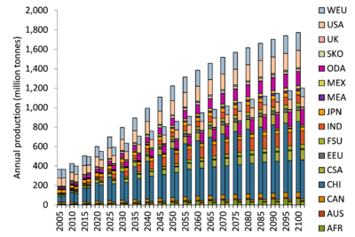 </figure>
<figure id="fig:Chemical">
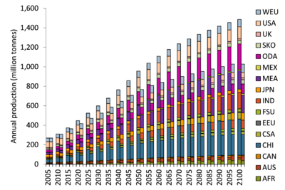 </figure>
<figure id="fig:Crop calorie production">
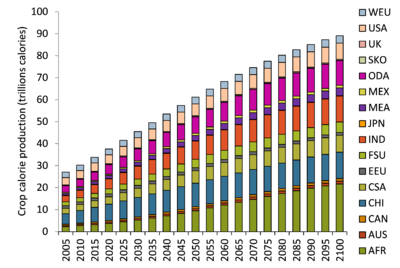
</figure>
3) Macro-economy - TIAM-UCL
The economy is represented for each region by hard-linking TIAM-UCL with Macro Stand Alone (MSA) module to allow consideration of the rest of the economy beyond energy i.e. general not partial equilibrium, and endogenises demand changes.
3.1) Production system and representation of economic sectors - TIAM-UCL
We have added a simplified general equilibrium macroeconomic growth module developed by Kypreos and Lehtila (2013). Macro Stand-Alone (MSA) is a single agent; single sector, multi-regional, general equilibrium optimal growth model which maximises discounted utility of a single consumer-producer agent. GDP is comprised of consumption, investment and energy system costs. Total economic production is determined by a combination of energy, capital and labour where energy substitutes with a capital-labour composite via an elasticity of substitution parameter. Quadratic cost functions and demand decoupling factors (essentially elasticity parameters for each period and demand)are estimated from the calibration routine are fed from TIAM-UCL to MSA. MSA is then solved and the new energy demands are given back into TIAM-UCL which is then solved again. The iteration continues until the model converges, defined by the change in energy service demand variation between interactions slowing to within a specified tolerance.
3.4) Trade - TIAM-UCL
Energy Trade
Regional trade is modelled in the trade module. In the current version of TIAM-UCL, regional trade is allowed for coal, natural gas, LNG, natural gas liquid, uranium oil and oil products such as heavy fuel oil, gasoline, naphtha, diesel, energy crops and solid biomass. Emission trading under cap-and-trade policy is also modelled and the level of trading can be constrained. Trading in the base-year 2005 is calibrated to the actual energy import and export data. Base-year energy trade (import and export of fossil resources) for the UK is taken from DUKES (2010).
Table 2-3: Resources traded in the 16 region TIAM-UCL global model
| Resource |
| Crude oil |
| Hard coal |
| Natural gas |
| Heavy fuel oil |
| Naphtha |
| Gasoline |
| Natural gas liquid |
| Distillates (diesel) |
| Liquefied natural gas |
| Uranium |
| Biomass |
| Bio-Fuels |
| Emissions permits |
4) Energy - TIAM-UCL
TIAM-UCL models all primary energy sources (oil, gas, coal, nuclear, biomass, and renewables) from resource production through to their conversion, infrastructure requirements, and finally to sectoral end-use. Note, throughout this section the term hurdle rate is used to refer to a technology specific discount rate. That is, the model assumes that the payment of any capital cost is spread over an economic life that may be different from the technical life of the process, and annualized at a different rate than the overall discount rate.
4.1) Energy resource endowments - TIAM-UCL
Fossil reserves and mining technologies are presented in the Table below on Non-renewable primary resources. A supply curve for each type of the sources shown is defined within region. Each time step is characterised by the cost of the resource and the total amount of energy available at this cost.
The Resource Module contains the data which separately characterises resources which are situated in regions with members of OPEC and those resources found in all other Non-OPEC regions. The module was originally based upon that provided in ETSAP-TIAM although significant changes have been made to their characterisation and dynamics of production including: adding Arctic oil and gas, shale gas and separately considering natural bitumen and kerogen oil produced by mining and by in situ methods. Geological constraints are also imposed upon oil and gas production that represent empirical depletion rate constraints.
Table: Non-renewable primary resources
| Technology Description |
| Oil |
| Existing proved plus probable reserves |
| Reserve growth |
| Undiscovered oil |
| Arctic oil |
| Natural bitumen ('oil sands') by in situ means of production |
| Natural bitumen ('oil sands') by mining |
| Extra-heavy oil |
| Kerogen oil by in situ means of production |
| Kerogen oil by mining |
| Natural gas liquids |
| Natural gas |
| Existing proved plus probable reserves |
| Reserve growth |
| Undiscovered gas |
| Arctic gas |
| Tight gas |
| Coal bed methane |
| Shale gas |
| Associated gas |
| Coal |
| Existing reserves |
| Additional resources |
| Uranium |
| Uranium (dummy) - Reserves |
4.1.3) Bioenergy - TIAM-UCL
Biofuels impact on land-use emissions are not considered and neither are life-cycle impacts of biofuels i.e. completely carbon neutral.
Biomass used in the electricity sector is provided by two different commodities - ELCSLD (from BIOSLD) and ELCCRP (from BIOCRP). Both originate from domestic (MIN) processes: MINBIOCRP0 (producing BIOCRP) and MINBIOSLD1,2 and 3 (producing BIOSLD). In this module biomass availability is modelled for energy crops and solid biomass (Table 11 5). Energy crops and solid biomass availability data is taken from TIAM-WORLD (www.kanors.com) and some adjustment made to match the regions in the TIAM-UCL. These two biomass resources are traded, transportation cost is presented in trade module. The domestic production bounds for 2005 can be found in the BY UPS templates. Concerning costs, all regions have the same COST for the three tranches of BIOSLD (at 0.63, 1.88 and 3.13). For BIOCRP, resource costs differ between regions although the basis for this differential is not clear. They range between 1.38 in India to 3.65 in ODA. All costs remain the same over the time horizon.
4.1.4) Non-biomass renewables - TIAM-UCL
Table 3.1.2 presents technology for renewable resources that are modelled in the TIAM-UCL. Renewable electricity resources such as hydro, geothermal, solar, tidal and wave are modelled. Solid biomass, energy crops, municipal waste and landfill gas are also modelled. Biomass technologies compete directly at energy service demand level with fossil fuel technologies. No distinction is made between OPEC and Non-OPEC countries for primary and secondary biomass production. Annual availability of renewable resources are controlled in different scenario files. Renewable production can be constrained through annual bounds on capacity and growth constraints.
Table 3.1.2: Renewable primary resources
| Technology Description |
| Hydro potential |
| Geothermal potential |
| Solar potential |
| Tide potential |
| Wind potential |
| Prod of Solid biomass |
| Prod of Industrial wastes |
| Prod of Municipal wastes |
| Prod of Gas from biomass (landfill gas) |
| Prod of Energy crop |
4.2) Energy conversion - TIAM-UCL
Energy conversion technologies in TIAM-UCL are undertaken by various distinct processes and are generally characterized by a number of data inputs including:
- investment costs
- operation and maintenance costs
- lifetime
- efficiency
- environmental outputs (CO2)
- growth constraints
Also, electricity grids are not explicitly modelled, with no capacity limits or investment requirements for system infrastructure. Two commodities are produced to represent generation from centralised (ELCC) and decentralised (ELCD) technologies. Distribution losses are modelled by commodity efficiency for ELCC (using parameter COM_IE). They reflect regional differences in the base year but by 2100 are the same across all regions. Electricity supply is tracked at a DAYNITE timeslice resolution. This allows for simplistic modelling of the load curve, representing when consumers demand electricity (see section 3 on demand drivers for more information). DAYNITE time-slices total 6 periods, representing day and night in the three (equal length) seasons (summer, winter, intermediate).
4.2.1) Electricity - TIAM-UCL
Conversion
The electricity and heat generation sector represents many different technology types, using a wide range of fossil-based and renewables resources. The existing system is represented in generic terms whilst the options for future investments are characterised in more detail. Annual electricity and heat supply is temporally disaggregated across six periods (or time slices), based on three season and two diurnal periods (Day / night) to represent changes in load based on sector demand profiles.
Electricity generation plant are additionally categorised as providing electricity to the centralised or decentralised grid (CEN or DCN). Decentralised producers tend to be small scale, connected to the distribution network or serving local grids, and produce one commodity in the model while centralised producers, connected to transmission network, produce a seperate commodity.
The electricity sector Base-Year template is used to calibrate the base-year electricity and heat generation. In the Base-Year template (providing information on existing plant), characterisation of plants is fairly generic, with all production of electricity categorised as ELC-CEN. Off-grid production (via micro-generation technologies) is not explicitly captured in the model, with small-scale generation represented in the decentralised producer group.
Figure: Existing Electricity Generation Capacity by Region in 2005 (Model base year), GW
Figure: Existing Electricity Generation Capacity by Type in 2005 (Model base year), GW
New technologies
Key technology options
New electricity generation technologies are listed in Table.
Table: New technology options for electricity
| Technology Group | Model Technology Description |
| Coal | Atmospheric Fl Bed. |
| Air Blown IGCC. | |
| Oxygen Blown IGCC. | |
| Pressurized Fl Bed. | |
| Pulverized Coal. | |
| Gas | Gas Steam. |
| Fuel Cells. | |
| Dual gas / oil | Gas_Oil Comb Cycle. |
| Advanced Gas_Oil Turbine. | |
| Oil | Oil Steam. |
| Generic Dist Gen for Base Load. | |
| Generic Dist Gen for Peak Load. | |
| Nuclear | Advanced Nuclear. |
| Fusion Nuclear. | |
| Advanced Nuclear LWR. | |
| Advanced Nuclear PBMR. | |
| Hydro* | Generic Impoundment Hydro. |
| Generic Impoundment Hydro. | |
| Generic Impoundment Hydro. | |
| Generic Impoundment Hydro. | |
| Generic Impoundment Hydro. | |
| Generic ROR Hydro. | |
| Biomass | Crop Direct Combustion. |
| Crop Gasification. | |
| Biogas from Waste. | |
| MSW Direct Combustion. | |
| Sld Biomass Direct Combustion. | |
| Sld Biomass Gasification. | |
| Sld Biomass Direct Combustion.Decentralized | |
| Sld Biomass Gasification.Decentralized | |
| Geothermal | Shallow. |
| Deep. | |
| Very deep. | |
| Solar PV* | CEN.PV.T0 |
| CEN.PV. | |
| CEN.PV.T1 | |
| CEN.PV.T2 | |
| CEN.PV.T3 | |
| CEN.PV.T4 | |
| CEN.PV.T5 | |
| DCN.PV.T0 | |
| DCN.PV. | |
| DCN.PV.T1 | |
| DCN.PV.T2 | |
| PV.T3 | |
| PV.T4 | |
| PV.T5 | |
| Solar thermal | CEN.Thermal. |
| Wind* | CEN. |
| CEN.Offshore. | |
| CEN.Onshore. | |
| DCN.Onshore. |
- Different tranches of renewable technologies represent differences in the cost of resources (hydro) or quality of the resource (wind, solar).
An important element is the transformation element which allows for regional differences to be introduced without having to duplicate technologies. For the electricity sector, the following parameters are controlled, and varied by region:
- Costs parameters (INVCOST, FIXOM and VAROM). Operation and maintenance costs tend to be lower in developing regions, as do investment cost where those regions have a technology manufacturing base e.g. China.
- Technology discount rate set to 10%, except for solar technologies, where the rate is higher for some regions. Higher rates are typically used for developing regions.
- Seasonal AFs are set by region for solar technologies, accounting for different insolation values.
- Construction time is provided for hydro and nuclear technologies - 10 years for nuclear and hydro (dam) and 5 years for hydro (run-of-river). No differentiation is made between regions.
Further work is required to include new CHP technologies, which are not available for public system or industry investment.
An overview of the key parameters for the different technology groups is shown in below.
Table: Overview of technology characteristics by technology group (for WEU region)
| Technology Group | Efficiency % (range) | Investment cost $/kW (range) | Comment | ||
| 2005 | 2050 | 2005 | 2050 | ||
| Coal | 40-49 | 40-49 | 1430-1870 | 1265-1662 | |
| Gas / Dual | 37-57 | 37-57 | 360-1000 | 300-1000 | Lower cost and higher efficiency values represent combined cycle technology |
| Oil | 31-35 | 31-35 | 660-1045 | 660-1045 | |
| Nuclear | 1760-1870 | 1760-1870 | Fusion costs set at 3300 $/kW | ||
| Hydro | 1650-6050 | 1540-5400 | Five dam-based technologies reflecting different cost of resource | ||
| Biomass | 33-34 | 33-34 | 1870-2200 | 1870-2200 | MSW plant significantly higher at 3850 $/kW |
| Geothermal | 1925-2780 | 1650-2310 | Three geothermal technologies reflecting different cost of resource | ||
| Solar PV | 7150-11000 | 1485-3025 | Low cost is centralised plant and high cost decentralised plant. Technology resource tranched on basis of AFs | ||
| Solar thermal | 13321 | 13321 | Single technology with no evolution on costs | ||
| Wind | 1065-1650 | 880-1310 | One backstop, one offshore (CEN) and 2 onshore (one is CEN and one is DCN) technologies. Offshore tech. represents the high costs. |
Power plants with CCS technologies
For low carbon analyses, sequestration technologies in the electricity generation sector are very important. The first five technologies listed have vintages for 2010, 2020 and 2030.
Table: Overview of Power plant with CCS technology characteristics
| Model Technology Description | Investment cost ($/kW) | Efficiency (%) |
| NGCC+Oxyfueling | 950-1250 | 48-55 |
| NGCC+CO2 removal from flue gas | 800-1000 | 49-57 |
| IGCC+CO2 removal from input gas | 1800-2300 | 40-48 |
| Conventional Pulverized Coal+Oxyfueling | 1900-2400 | 37-44 |
| Conventional Pulverized Coal+CO2 removal from flue gas | 1850-2250 | 38-44 |
| SOFC (COAL) +CO2 removal - 2030 | 2200 | 48 |
| SOFC (GAS) +CO2 removal - 2020 | 1600 | 58 |
| Crop Direct Combustion. With CCS | 2125 | 33 |
| Crop Gasification.with CCS | 2500 | 34 |
| Sld Biomass Direct Combustion.with CCS | 1700 | 33 |
| Sld Biomass Gasification.with CCS | 2420 | 34 |
The fossil-based plants produce SNKELCCO2, a 'dummy' commodity which then goes to the different storage technologies. Biomass plants with sequestration produce SNKTOTCO2, differentiated as technologies that capture CO2 from the atmosphere (negative emissions). The range of storage technologies in the model are listed below.
Types of storage technologies
Removal by Enhanced Coalbed Meth recov <1000 m
Removal by Enhanced Coalbed Meth recov >1000 m
Removal by Depl gas fields (offshore)
Removal by Depl gas fields (onshore)
Removal by Storage in the deep ocean
Removal by Depl oil fields (offshore)
Removal by Depl oil fields (onshore)
Removal by Deep saline aquifers
Removal by Enhanced Oil Recovery
Mineralization for CO2 storage
4.2.2) Heat - TIAM-UCL
Heat technologies are respresented as
- Public CHP plant, providing electricity to the grid and heat to local distict heating networks
- Sector CHP plant (autoproducers), providing electricity and heat to specific industries.
- Public heat generation plant (heat only plants), providing heat to local distribution networks
4.2.3) Gaseous fuels - TIAM-UCL
Alternative fuels
Table 3.2.4 contains technologies for the production of alternative fuels. The technologies are split into two groups: 1) Ethanol and methanol production, either from coal or biomass and 2) Fischer-Tropsch processes, producing oil products from coal, gas and biomass.
Table 3.2.4: Alternative fuel technologies
| Model Technology Description |
| Ethanol from biomass |
| Cellulose ethanol plant |
| Methanol from Bioliquids |
| Methanol from coal |
| Methanol from coal with CO2 capture |
| Methanol from natural gas |
| Methanol from natural gas with CCS |
| FT fuels from natural gas |
| FT fuels from natural gas with CCS |
| FT fuels from coal |
| FT fuels from coal with CCS |
| FT fuels from coal low biomass and coal co production |
| FT fuels low biomass and coal co production with CCS |
| FT fuels high biomass and coal co production |
| FT fuels high biomass and coal co production with CCS |
| FT fuels solid biomass |
| FT fuels solid biomass with CCS |
Hydrogen
New technologies include those used for hydrogen production and demand technologies in the transport sector that consume hydrogen. Production technologies are generic in nature and are defined by the type of fuel used - coal, natural gas, electricity and biomass.
There are also technologies, available from 2020, that allow for mixing of hydrogen into the natural gas supply to different sectors. This mix is fixed at 15% hydrogen / 85% natural gas. A single distribution technology allows for hydrogen transport, with costs developed on the basis of unit of energy transported (using VAROM).
Table 3.2.5: Hydrogen production and supply technologies
| Model Technology Description |
| Hydrogen from Brown coal |
| Hydrogen from Hard coal |
| Electrolysis |
| Hydrogen from NGA |
| Hydrogen from NGA - Decentralized |
| Hydrogen from biomass gasification |
| Mix of Gas and Hydrogen - For COM |
| Mix of Gas and Hydrogen - For IND |
| Mix of Gas and Hydrogen - For RES |
| Distribution of hydrogen |
Hydrogen technologies for cars and light duty trucks are included in the model, with different types based on the use of combustion, hybrid or fuel cell technology. The associated Trans file puts different hurdle rates on these technologies, assuming 15% for developed regions and 30% for developing regions such as Africa. The Trans file is also used to adjust efficiencies and costs across all regions, for both transport and production technologies.
Sequestration
Sequestration technologies and storage options mainly relate to the electricity sector, and are described in the relevant sector chapter of this report.
There are two technologies that allow for the capture of CO2 emissions (process-based) in the upstream sector. The costs of such 'dummy' capture technologies are modelled simply, using variable costs of 0.001 (equivalent to $1/tCO2).
Another set of important technologies for integrated climate modelling are those that relate to emissions and removals by the forestry sector. Labelled SINKAF*. The levels of emissions and removals and the associated costs are controlled by the Trans file and are based on assumptions used in the EMF analysis. Finally, atmospheric CO2 may be partly absorbed and fixed by biological sinks such as forests; the model has six options for forestation and avoided deforestation, as described in Sathaye et al. (2005) and adopted by the Energy Modelling Forum, EMF-21 and 22 groups.
Land-use CO2
The SubRes file LUCO2 defines a single technology that emits fixed levels of emissions by region each period. It is net CO2 emissions from deforestation and forest degradation. It does not include emissions from land use. The levels are calculated in the associated Trans file. The global emission level in 2005 is estimated at 2.7 GtCO2 per year, which decreases to 0.1 GtCO2 by 2100.Allocation by region is based on distribution of agricultural managed land. It is assumed that LULUCF emissions for UK is zero and therefore, WEU region's LULUCF emission has not been changed. There are scenarios in the model with reduced emissions from deforestation based on the EMF 21 study scenarios.
Grid and infrastructure
No representation of grids in TIAM-UCL except Electricity generation can be centralised or decentralised (CEN or DCN). A generic cost and efficiency loss associated with distribution are included for Gas pipelines and electricity.
The range of CO2 storage technologies in the model are listed below.
Table 3.2.6: Types of storage technologies
| Model Technology Description |
| Removal by Enhanced Coalbed Meth recov <1000 m |
| Removal by Enhanced Coalbed Meth recov >1000 m |
| Removal by Depl gas fields (offshore) |
| Removal by Depl gas fields (onshore) |
| Removal by Storage in the deep ocean |
| Removal by Depl oil fields (offshore) |
| Removal by Depl oil fields (onshore) |
| Removal by Deep saline aquifers |
| Removal by Enhanced Oil Recovery |
| Mineralization for CO2 storage |
4.3) Energy end-use - TIAM-UCL
Energy end-use demand is broken down into the following sectors: Transport, Residential and Commercial, Industry and Other (Agriculture). Each sector is composed of a number of energy service demands that map to specific components of that sector, e.g. residential hot water. The temporal trajectory of these energy service demands are linked to underlying demand drivers such as GDP or population, as will be detailed later (see Energy demand - TIAM-UCL).
4.3.1) Transport - TIAM-UCL
Energy services demand
The transportation sector is characterized by 14 energy-services plus one non-energy use demand segment (Table 3.3.1). Six of the energy-services are considered as generic demands: international and domestic aviation, freight and passenger rail transportation, domestic and international navigation. All other energy-services are for road transport. The non-energy use is predominately the demand lubricants. Demand for road transport energy-services is expressed in billion vehicle km (b-vkm) and others are in PJ. The model projects energy-services demands for each region.
Table 3.3.1: Energy-service demands in transport sector
| Energy-service sectors |
| Domestic Aviation |
| International Aviation |
| Road Bus Demand |
| Road Commercial Trucks Demand |
| Road Three Wheels Demand |
| Road Heavy Trucks Demand |
| Road Light Vehicle Demand |
| Road Medium Trucks Demand |
| Road Auto Demand |
| Road Two Wheels Demand |
| Rail-Freight |
| Rail-Passengers |
| Domestic Internal Navigation |
| International Navigation |
| Non-energy use |
Table 3.3.2 presents the list of transport fuels available to meet the base-year energy-service demand in each transport subsector. Diesel and gasoline are considered as the conventional fuels and the other are alternative fuels which are introduced later. Jet fuel and electricity are available to meet aviation demand.
Table 3.3.2: transport fuels
| Fuel |
| diesel |
| electricity |
| ethanol |
| gasoline |
| LPG |
| methanol |
| natural gas |
For each end-use, a number of new (i.e. available after the base year of 2005) technologies are in competition to satisfy the energy-services demand for future years. Efficiency and cost of these technologies improve over the period with vintages. These technologies progressively replace the existing ones (i.e. those used in the base year) and they are characterized by the same type of parameters such as efficiency, and investment cost. There are many new technologies available for the road transport sector whereas technological detail is very limited in rail, shipping and aviation modes. Investment and O&M costs shown are US dollar reference prices. They are multiplied by regionally specific factors for each region. Technology and regional specific hurdle rates, which are used to annualise the investment cost, are also applied.
As an outcome of the ADVANCE project, TIAM-UCL can now explicitly distinguish up to 27 different types of vehicle users (e.g., urban or rural, frequent or less frequent, risk averse or novelty-seeking). Non-financial vehicle attributes including novelty, range, and refueling availability can also now influence vehicle choices in an explicit way. Consumers' preferences for these attributes have been monetized drawing on the expertise of a detailed transport sector model (MA3T). These 'intangible' costs and benefits have been included alongside pure financial costs in the investment cost calculations influencing vehicle choice. Importantly, these additional terms vary uniquely by consumer type, by region, and by vehicle technology.
4.3.2) Residential and commercial sectors - TIAM-UCL
Residential sector
Residential sector final energy consumption calibration is carried out in the Base-Year template for residential, commercial and agriculture sectors. The template uses IEA residential sector final consumption data for the base-year 2005. It also includes details for residential sector fuels and all existing technologies in residential sector. The template also captures residential sector emissions. All new technologies that are available after the first year (base-year) are modelled separately. Selected energy-services in the residential sector also have demand data at the sub-regional level for certain regions in order to have different growth rates.
Energy service demands
The residential sector includes 11 energy-services as presented in Table 3-4-3. All energy-service demands are in PJ. In the residential sector, some segments are identified using more than one abbreviation, which means that the demand can be disaggregated in four or less sub-regions. Currently, USA and CAN have four and three geographic regions, respectively, while AFR, CHI, IND, MEA and MEX each have two sub-regions, corresponding to rural and urban areas. When no sub-regions have been defined, the abbreviation for sub-region 1 is used by default. Energy service demands are projected to 2100 using general economic and demographic drivers (population, GDP and GDP per capita). To develop projections of future energy-service demands, estimates of drivers are used in conjunction with user assumptions on the topic of service demand sensitivity to these drivers (see Section on demand projections and drivers). Growth rates for residential lighting are relatively high in selected sub-regions in the developing world. This is because of very low level of electrification at present (base-year) in these sub-regions.
Table 3.4.3: Residential sector energy-services
| Energy-Service |
| Residential Cooling |
| Residential Clothes Drying |
| Residential Clothes Washing |
| Residential Dishwashing |
| Residential Other Electric |
| Residential Space Heat |
| Residential Hot Water |
| Residential Cooking |
| Residential Lighting |
| Residential Refrigeration |
| Residential Others |
The same fuels (both Existing and New) are used in both the Residential and Commercial sectors.
Technologies
Residential sector existing end-use technologies are modelled in the Base-Year templates. No investment can be made in existing technologies. New technologies progressively replace the existing ones as they reach the end of their technology life assumptions. For each end-use energy-service, a number of existing technologies are in competition to satisfy the demand. They are characterized by an efficiency, an annual utilization factor, a lifetime, operation costs, and six seasonal share coefficients (summer-day, summer-night, intermediary-day, intermediary-night, winter-day, winter-night). The sum product of the final energy consumption and the efficiency of technologies give the base-year demand value. Region specific hurdle rates, which are used to annualise investment cost of the residential end-use technologies, has been applied to residential sector technologies.
Commercial Sector
Commercial sector base-year final energy consumption is calibrated in the residential sector Base-Year template, which has separate work sheets for commercial sector IEA data, sector fuel data, end-use technology data and emissions data. There are separate sheets available for technology data for each energy-service demand.
Energy services demand
The commercial sector includes eight energy service demands for each region as presented in Table 3.4.1. Some segments of the commercial sector energy-services are identified using more than one code, which means that the demand can be disaggregated in four or less sub-regions.When no sub-regions have been defined, the codes for sub-region 1 are used by default. Currently, USA and CAN have four and three geographic regions, respectively, while AFR, CHI, IND, MEA and MEX each have two sub-regions, corresponding to rural and urban areas. The energy-service demands for the future period (2005-2100) are projected using appropriate drivers and elasticities.
Table 3.4.1: Energy-services in commercial sector
| Energy-service |
| Commercial Cooling |
| Commercial Cooking |
| Commercial Space Heat |
| Commercial Hot Water |
| Commercial Lighting |
| Commercial Office Equipment |
| Commercial Refrigeration |
Sector fuels
Table 3.4.2 contains details of existing fuel technologies (each also has a new fuel technology vintage) for the commercial sector. Commercial sector emissions factor to capture commercial sector emissions are also included in the Base-Year template.
Table 3.4.2: commercial sector fuel technologies-existing
| Technology Description |
| Fuel Tech - Natural Gas Mix (COM) |
| Fuel Tech - Diesel (COM) |
| Fuel Tech - Heavy Fuel Oil (COM) |
| Fuel Tech - Kerosene (COM) |
| Fuel Tech - Coal (COM) - Existing |
| Fuel Tech - Liquefied Petroleum Gases (COM) |
| Fuel Tech - Biofuels (COM) |
| Fuel Tech - Geothermal (COM) |
| Fuel Tech - Solar (COM) |
| Fuel Tech - Electricity (COM) |
| Fuel Tech - Heat (COM) |
Technologies
There are a number of existing technologies modelled for each energy service demand in the Base-Year template for each region and sub-region. For each energy service demand, a number of technologies are in competition to satisfy the demand. They are characterized by an efficiency, an annual utilization factor, a lifetime, operation costs, and six seasonal share coefficients (summer-day, summer-night, intermediary-day, intermediary-night, winter-day, winter-night). A list of new technologies are modelled. These technologies are available after the first period (base-year) and progressively replace the existing ones as they reach the end of their technology life assumptions. In addition to parameters specified for existing technologies, new technology descriptions include information such as technology cost. The parameters such as cost, efficiency, etc., can improve over the years with vintages. Regional specific hurdle rates, which is used to annualised the investment cost, are used for commercial end-use technologies.
4.3.3) Industrial sector - TIAM-UCL
Energy-service demands
The industrial sector is characterized by 6 demand segments, each representing either the physical output of the industry or the total energy requirement (Table 3.5.1). There are also one demand for 'Other non-specified energy consumption (ONO)', one for 'Industrial and Other non-energy uses (NEO)' and one for 'Other Industrial consumption (I0I)', which are considered as a generic demands. The last one (I0I) has been added for minor calibration purposes and is generally not used. There are different technologies and fuels modelled for supplying steam, process heat, machine drives and electro-chemical process for each energy-service demand in the Base-year templates.
Table 3.5.1: Industry sector energy-services
| Code | Energy-service demand | Unit |
| I0I | Other Industrial consumption | PJ |
| ICH | Chemicals | PJ |
| IIS | Iron and Steel | Mt |
| ILP | Pulp and Paper | Mt |
| INF | Non-ferrous metals | Mt |
| INM | Non Metals | PJ |
| NEU | Other Industries | PJ |
| NEO | Industrial and Other Non Energy Uses | PJ |
| ONO | Other non-specified consumption | PJ |
Energy service demands are projected to 2100 using general economic and demographic drivers population, GDP, GDP per capita and sectoral output). To develop projections of future energy service demands, estimates of drivers are used in conjunction with user assumptions on the topic of service demand sensitivity to these drivers. Projected industry sector energy-service demands at a global level are presented in Figure 3.5.1. Similar tables have been generated for each region. Industry sector has relatively high growth in China as compared to other regions.
Figure 3.5.1: projected industry sector energy-service demands at global level
There are hundreds of technologies modelled in the industry sector to meet the energy-service demands. For each energy-services of each industry, a number of existing technologies are in competition to satisfy energy-service demand. They are characterized by an efficiency, an annual utilization factor, a lifetime, operation costs, and six seasonal share coefficients (summer-day, summer-night, intermediary day, intermediary-night, winter-day, winter-night). The technologies included in the Base-Year template are the existing technologies to meet the base-year demand and the residual capacities can be used till end of their life period. No new investments are allowed in the existing technologies in any sector. . These technologies progressively replace the existing ones and they are characterized by the same type of parameters such as efficiency, and investment cost. Regional specific hurdle rates are applies to industry sector new technologies as shown in Figure 3.5.2. It varies from 10% (developed countries) to 20% (least developed countries).
Figure 3.5.2: Regional specific hurdle rate for industry sector technologies
4.3.4) Other end-use - TIAM-UCL
Agriculture
Energy services demand
Energy-service demand in the agricultural sector is represented by a single demand segment and projected using the driver 'agricultural sector output', which is based on GDP per capita and population, for each region. Figure 3.6.1 presents the projected energy-service demand by region. Note that there are no new technologies associated with the generic demand (AGR). In this sector, it is assumed that increases in agricultural output result in proportionate increases in energy input.
Figure 3.6.1: Agriculture energy-service demand projection by region
Sector fuels
Sectoral fuel technologies are modelled in the sheet AGR_Fuels in the residential Base-Year template as shown in Table 3.6.1. The fuels are aggregated into 13 categories consumed in the agriculture sector. Aggregation ratios are based on data provided by the IEA database. The technologies created to produce aggregated fuels (Fuel Tech) are named uniformly using the name of the aggregated fuels as specified in the column Commodity OUT plus three zero (000 for existing technology in the base-year). Their description changes according to the fuel (e.g. Fuel Tech - Coal (AGR) or Fuel Tech - Natural Gas (AGR). The fractional shares of the disaggregated fuels (Commodity IN) used to produce an aggregated fuel (Commodity OUT) are calculated from their consumption over the total for this category, as given in the IEA database.
Table 3.6.1: Agriculture sector fuel technologies-existing
| Technology Description |
| Fuel Tech - Natural Gas Mix (AGR) |
| Fuel Tech - Natural Gas (AGR) |
| Fuel Tech - Diesel (AGR) |
| Fuel Tech - Gasoline (AGR) |
| Fuel Tech - Heavy Fuel Oil (AGR) |
| Fuel Tech - Kerosene (AGR) |
| Fuel Tech - Coal (AGR) |
| Fuel Tech - Liquified Petroleum Gases (AGR) |
| Fuel Tech - Biofuels (AGR) |
| Fuel Tech - Geothermal (AGR) |
| Fuel Tech - Solar (AGR) |
| Fuel Tech - Electricity (AGR) |
| Fuel Tech - Heat (AGR) |
Base-year calibration
IEA energy balance provides agriculture energy consumption by fuels. Since agriculture sector is defined with a single energy-service, there is no need for that split of fuel consumptions into different sub-sector as we did for other end-use sector. Fuels in the IEA energy balance has been aggregated into 13 fuels (commodity) as defined in the sector fuel table (Table 3.6.1). The energy mix of Base-year global agriculture final energy consumption (7,283 PJ) is presented in Figure 3.6.2 at a global level.
Figure 3.6.2: Base-year agriculture energy consumption mix by fuel
4.4) Energy demand - TIAM-UCL
Demand drivers (population, GDP, family units, etc.) are obtained externally, via other models or from other sources (e.g. UN statistics, World Bank, IEA). Energy-service demands and respective drivers in the TIAM-UCL are presented in Table 2-1. The demands for energy services are linked to the drivers' projections via elasticities, see bellow. These elasticities of demands are intended to reflect changing patterns in energy service demands in relation to socio-economic growth, such as saturation in some energy end-use demands, increased urbanization, or changes in consumption patterns once the basic needs are satisfied. The energy-service demands for future years are projected using the following relationship:
Where k is a constant equal to 1 for most of the energy services demand. The constant k is population and number of households when the driver is GDP per Person (GDPP) and GDP per Household (GDPPHOU) respectively.
Table 2-1: Energy-services demand and respective drivers
| Code | Description | Unit | Driver |
|---|---|---|---|
| ICH | Chemicals | PJ | PCHEM |
| IIS | Iron and Steel | Mt | PISNF |
| INF | Non-ferrous metals | Mt | PISNF |
| INM | Non Metals | PJ | POEI |
| ILP | Pulp and Paper | Mt | POEI |
| IOI | Other Industries | PJ | POI |
| I00 | Other Industrial consumption | PJ | Constant |
| NEO | Industrial and Other Non Energy Uses | PJ | GDP |
| ONO | Other non-specified consumption | PJ | GDP |
| AGR | Agricultural demand | PJ | PAGR |
| CC1 | Commercial Cooling - Region 1 | PJ | PSER |
| CCK | Commercial Cooking | PJ | PSER |
| CH1 | Commercial Space Heat - Region 1 | PJ | PSER |
| CHW | Commercial Hot Water | PJ | PSER |
| CLA | Commercial Lighting | PJ | PSER |
| COE | Commercial Office Equipment | PJ | PSER |
| CRF | Commercial Refrigeration | PJ | PSER |
| RC1 | Residential Cooling - Region 1 | PJ | HOU/GDPPHOU* |
| RCD | Residential Clothes Drying | PJ | HOU/GDPPHOU* |
| RCW | Residential Clothes Washing | PJ | HOU/GDPPHOU* |
| RDW | Residential Dishwashing | PJ | HOU/GDPPHOU* |
| REA | Residential Other Electric | PJ | HOU/GDPPHOU* |
| RH1 | Residential Space Heat - Region 1 | PJ | HOU |
| RHW | Residential Hot Water | PJ | POP |
| RK1 | Residential Cooking - Region 1 | PJ | POP |
| RL1 | Residential Lighting - Region 1 | PJ | GDPP |
| RRF | Residential Refrigeration | PJ | HOU/GDPPHOU* |
| NEU | Non Energy Uses | PJ | GDP |
| TAD | Domestic Aviation | PJ | GDP |
| TAI | International Aviation | PJ | GDP |
| TRB | Road Bus Demand | Bv-km | POP |
| TRC | Road Commercial Trucks Demand | Bv-km | GDP |
| TRE | Road Three Wheels Demand | Bv-km | POP |
| TRH | Road Heavy Trucks Demand | Bv-km | GDP |
| TRL | Road Light Vehicle Demand | Bv-km | GDP |
| TRM | Road Medium Trucks Demand | Bv-km | GDP |
| TRT | Road Auto Demand | Bv-km | GDPP |
| TRW | Road Two Wheels Demand | Bv-km | POP |
| TTF | Rail-Freight | PJ | GDP |
| TTP | Rail-Passengers | PJ | POP |
| TWD | Domestic Internal Navigation | PJ | GDP |
| TWI | International Navigation | PJ | GDP |
- The driver is GDPPHOU for AFR, CHI, CSA, EEU, FSU, IND, MEA, MEX, ODA and SKO
Driver Elasticity
Driver elasticities determine the sensitivity of changes in energy-service demand to changes in the underlying driver. An elasticity of 1 means that a change of the underlying driver is exactly reflected in the energy-service demand. Energy-service demands with an elasticity below 1 are demand inelastic, while those with an elasticity of one or higher are demand elastic. In general it is assumed that energy-service demands grow slower than the underlying driver, such as GDP, GDP per capita or number of household. This decoupling of energy demand and economic growth is expected to increase during the 21st century so that all elasticities fall. Residential space heating (RH1), for example, has an elasticity of 0.8 in 2010, which drops to 0.5 in 2100. This means that initially the energy demand for space heating increases at 80% of household number growth, the specific underlying driver, and in the 2nd half of the century at only 50% of the household number growth rate.
Table 2-2: Driver elasticities for the United Kingdom
| Energy-service demand | 2010 | 2020 | 2030 | 2040 | 2050 | 2100 |
| AGR | 0.8 | 0.8 | 0.8 | 0.8 | 0.8 | 0.6 |
| CC1 | 0.8 | 0.8 | 0.8 | 0.8 | 0.7 | 0.4 |
| CCK | 0.5 | 0.5 | 0.5 | 0.5 | 0.5 | 0.4 |
| CH1 | 0.5 | 0.5 | 0.5 | 0.5 | 0.5 | 0.3 |
| CHW | 0.5 | 0.5 | 0.5 | 0.5 | 0.5 | 0.4 |
| CLA | 0.5 | 0.5 | 0.5 | 0.5 | 0.5 | 0.4 |
| COE | 0.5 | 0.5 | 0.5 | 0.5 | 0.5 | 0.4 |
| COT | 0.5 | 0.5 | 0.5 | 0.5 | 0.5 | 0.4 |
| CRF | 0.5 | 0.5 | 0.5 | 0.5 | 0.5 | 0.4 |
| I00 | 0.6 | 0.6 | 0.6 | 0.6 | 0.6 | 0.5 |
| ICH | 0.8 | 0.8 | 0.8 | 0.8 | 0.7 | 0.5 |
| IIS | 0.7 | 0.7 | 0.7 | 0.7 | 0.7 | 0.5 |
| ILP | 0.8 | 0.8 | 0.8 | 0.8 | 0.7 | 0.5 |
| INF | 0.8 | 0.8 | 0.8 | 0.8 | 0.7 | 0.5 |
| INM | 0.8 | 0.8 | 0.8 | 0.8 | 0.7 | 0.5 |
| IOI | 0.8 | 0.8 | 0.8 | 0.8 | 0.8 | 0.6 |
| NEO | 0.6 | 0.6 | 0.6 | 0.6 | 0.6 | 0.5 |
| NEU | 1 | 1 | 1 | 1 | 0.9 | 0.5 |
| ONO | 0.6 | 0.6 | 0.6 | 0.6 | 0.6 | 0.5 |
| RCD | 1 | 1 | 1 | 1 | 1 | 0.8 |
| RCW | 1 | 1 | 1 | 1 | 1 | 0.8 |
| RDW | 1 | 1 | 1 | 1 | 1 | 0.8 |
| REA | 1 | 1 | 1 | 1 | 1 | 0.8 |
| RH1 | 0.8 | 0.8 | 0.8 | 0.8 | 0.8 | 0.5 |
| RK1 | 0.7 | 0.7 | 0.7 | 0.7 | 0.7 | 0.5 |
| RL1 | 1 | 1 | 1 | 1 | 0.9 | 0.7 |
| ROT | 1 | 1 | 1 | 1 | 1 | 0.8 |
| RRF | 1 | 1 | 1 | 1 | 1 | 0.8 |
| RHW | 1 | 1 | 1 | 1 | 1 | 0.8 |
| TAD | 1.2 | 1.2 | 1.1 | 1.1 | 0.9 | 0.1 |
| TAI | 1.2 | 1.2 | 1.1 | 1.1 | 0.9 | 0.1 |
| TRB | 0.7 | 0.7 | 0.7 | 0.7 | 0.7 | 0.8 |
| TRC | 0.7 | 0.7 | 0.7 | 0.7 | 0.7 | 0.4 |
| TRE | 0.7 | 0.7 | 0.7 | 0.7 | 0.7 | 0.7 |
| TRH | 0.7 | 0.7 | 0.7 | 0.7 | 0.7 | 0.4 |
| TRL | 0.7 | 0.7 | 0.7 | 0.7 | 0.7 | 0.4 |
| TRM | 0.7 | 0.7 | 0.7 | 0.7 | 0.7 | 0.4 |
| TRT | 1.2 | 1.2 | 1.2 | 1.2 | 1 | 0.5 |
| TRW | 0.7 | 0.7 | 0.7 | 0.7 | 0.7 | 0.7 |
| TTF | 1 | 1 | 1 | 0.8 | 0.6 | 0.1 |
| TTP | 0.8 | 0.8 | 0.8 | 0.8 | 0.8 | 0.7 |
| TWD | 0.8 | 0.8 | 0.8 | 0.6 | 0.5 | 0.1 |
| TWI | 0.8 | 0.8 | 0.8 | 0.6 | 0.5 | 0.1 |
Non-energy demands are not explicitly considered.
Regional GDP per capita is a driver for the model, but there are no income distribution within a given region. Access issues are not considered either.
Regions can be split to additional subregions for the demand level, thus allowing to model demand separately for, for example, urban and rural areas in the Residential sector. Currently, USA and CAN have four and three geographic regions, respectively, while AFR, CHI, IND, MEA and MEX each have two ?sub-regions?, corresponding to rural and urban areas.
Behavioural change
Behaviour and heterogeneous agents are mostly not explicitly considered but are represented via price mechanisms e.g. there is no modal shift in the transport sector. With the exceptions of technology and region specific discount rates and price responsive energy service demands i.e. see Residential sector. Diffusion constraints can be implemented to simulate behavioural inertia (among the other barriers that are not explicitly included in the model).
4.5) Technological change in energy - TIAM-UCL
TIAM-UCL represents technological change through exogenously determined cost-reductions and efficiency improvements for the various different technologies available, although learning curves have also been used in specific studies. However, R&D expenditures are not explicitly considered.
Technology vintages are fully represented and explicit growth and decline constraints can be used to simulate the diffusion and phase out of technologies.
Representation of inertias and path-dependencies, e.g. via capacity stocks, knowledges stocks (cf. technological change), constraints of the expansion and decline of technology deployment, and early retirements of fossil capacities are all included.
Endogenous technological learning is also possible.
5) Land-use - TIAM-UCL
No land-use representation in TIAM -UCL except for land-use emissions from the agriculture sector.
6) Emissions - TIAM-UCL
In the sub-sections of this chapter, the GHG and non-GHG emissions included in TIAM-UCL are presented.
6.1) GHGs - TIAM-UCL
Carbon dioxide, Methane and Nitrous Oxide are all modelled in TIAM-UCL and these are linked to each individual technology.
TIAM includes energy related CO2, land-use (and forestry) CO2, and non-CO2 gases CH4 and N2O. CH4 from upstream, landfills, manure, rice paddies, enteric fermentation, wastewater is based on EMF-22 data and WEO-2008. N2O from industry and agriculture is based on WEO-2008. CO2 from land-use is based on the Reference scenario of the United States Climate Change Science Program (MIT) presented in Prinn et al. (2008). UK data for Non-CO2 gases are taken from UK greenhouse gas inventory national system (www.ghgi.org.uk).
Some other greenhouse gases (CFCs, HFCs, SF6, etc.) and chemically active gases such as NOX, CO, VOCs are not explicitly modelled, but their radiative forcing is represented as an exogenous extra term in the Forcing expression (this is only for climate module). When aggregate non-CO2 emissions (CH4 and N2O) to CO2 equivalent, the model uses a factor of 0.025 for CH4 and 0.298 for N2O.
The emissions accounting for non-CO2 emission sources are listed in Table 5.1 below. These emission sources are important to include when running climate targets taking account of all GHGs. Emission levels are exogenously determined using EMF data.
'Table 5.1: Non-CO'2 emission sources
| Sector | Emission source | GHG |
| Industry | Adipic Acid Production | N2O |
| Industry | Nitric Acid Production | N2O |
| Agriculture | Manure | CH4 |
| Agriculture | Other e.g. residue burning | CH4 |
| Agriculture | Other | N2O |
| Residential | Landfill | CH4 |
| Residential | Other e.g. wastewater | CH4 |
6.2) Pollutants and non-GHG forcing agents - TIAM-UCL
Pollutants and non-GHG forcing agents are not explicitly modelled, however additional forcing factor are included in the climate module.
7) Climate - TIAM-UCL
The climate module is a simplification of the climate system incorporating emissions of three major greenhouse gases (carbon dioxide, methane and nitrous oxide) to calculate radiative forcing and temperature changes. The results of the climate system (temperature change) can been linked to simplified damage functions to calculate future costs brought by climate change. We have extracted damage functions from the integrated assessment model PAGE09 (Hope 2011). After a recalibration of the climate module of TIAM-UCL using the latest version of the MAGICC climate model (Meinshausen et al. 2011), we have matched data from the 8 regions within PAGE onto the 16 regions included within TIAM-UCL to produce the climate module
The climate module uses emissions that are endogenously calculated in TIAM as an input. These are carbon dioxide (CO2), methane (CH4) and nitrous oxide (N20). Successively, it calculates changes in the concentration of CO2, CH4 and N2O, change in radiative forcing over pre-industrial times from all three gases plus an exogenously defined additional forcing and finally the temperature change over pre-industrial times for the atmosphere and the deep ocean. Figure 5.1 gives a graphical overview of the modules structure.
The underlying mathematical structure of the module is based on a linear recursive approach from Nordhaus and Boyer (1999). This is a well-documented, albeit simple approach, which gives a good approximation of more complex climate models (Loulou et al. 2010, p. 3).
Instead of converting non-CO2 greenhouse gases into CO2-equivalents and calculating concentrations and radiative forcing on this basis, the module models the life cycle of each endogenous emission separately.
Figure 5.1: Illustration of the TIAM climate module <figure id="fig:climate_module.png">
8) Non-climate sustainability dimension - TIAM-UCL
In TIAM-UCL, non-climate sustainability is not currently modelled.
9) Appendices - TIAM-UCL
10) References - TIAM-UCL
Clarke, L., J. Edmonds, H. D. Jacoby, H. Pitcher, J. M. Reilly and R. Richels (2007): Scenarios of Greenhouse Gas Emissions and Atmospheric Concentrations. Sub-report 2.1A of Synthesis and Assessment Product 2.1 by the U.S. Climate Change Science Program and the Subcommittee on Global Change Research. Department of Energy / Office of Biological & Environmental Research. Washington, DC.: 154.
Dessens O. and Anandarajah G. (2012) Soft coupling between the integrated assessment models PAGE and TIAM-UCL: climate change damage function and greenhouse gas emissions abatement costs. IEW2012, Cape Town, South Africa, June 19-21.
Forster, P., V. Ramaswamy, P. Artaxo, T. Berntsen, R. Betts, D.W. Fahey, J. Haywood, J. Lean, D.C. Lowe, G. Myhre, J. Nganga, R. Prinn, G. Raga, M. Schulz and R. Van Dorland, 2007: Changes in Atmospheric Constituents and in Radiative Forcing. In: Climate Change 2007: The Physical Science Basis. Contribution of Working Group I to the Fourth Assessment Report of the Intergovernmental Panel on Climate Change [Solomon, S., D. Qin, M. Manning, Z. Chen, M. Marquis, K.B. Averyt, M.Tignor and H.L. Miller (eds.)]. Cambridge University Press, Cambridge, United Kingdom and New York, NY, USA.
Hope, C. (2011) The PAGE09 integrated assessment model: A technical description. Cambridge Judge Business School Working Paper. Cambridge, UK.
International Energy Agency (IEA), World Energy Balances, 2009, ESDS International, (Mimas) University of Manchester
Kypreos, S. and A. Lehtila (2013), TIMES-Macro: Decomposition into Hard-Linked LP and NLP problems, ETSAP TIMES 3.4 User Note, 25 March 2015
Lehtila A., Loulou R. (2005) TIMES Damage Functions. ETSAP TIMES Version 2.0 User Note. IEA-ETSAP.
Loulou, R., and M. Labriet (2007), ?ETSAP-TIAM: The TIMES Integrated Assessment Model --Part I: Model Structure?, Computational Management Science special issue on Energy and Environment, Vol. 5, No 1-2, pp. 7-40
Loulou, R., Lehtila, A., Labriet, M. (2010): ?TIMES Climate Module (Nov. 2010)?, ETSAP, http://www.etsap.org/documentation.asp
Morita, Tsuneyuki (1999) Emission Scenario Database prepared for IPCC Special Report on Emission Scenarios convened by Dr. Nebosja Nakicenovic, National Institute for Environmental Studies Centre for Global Environmental Research
Meinshausen M., Raper S. C. B. and Wigley T. M. L. (2011) Emulating coupled atmosphere-ocean and carbon cycle models with a simpler model, MAGICC6 ? Part 1: Model description and calibration. Atmospheric Chemistry and Physics 11(4): 1417-1456.
Nordhaus, W.D., Boyer, J. (1999): ?Roll the DICE Again: Economic Models of Global Warming?, Yale University, manuscript edition.
Prinn R., S. Paltsev, A. Sokolov, M. Sarofim, J. Reilly, and H. Jacoby (2008). The Influence on Climate Change of Differing Scenarios for Future Development Analyzed Using the MIT Integrated Global System Model. Report nยบ163, MIT Joint Program on the Science and Policy of Global Change, 32 p.
Ramaswamy, V., Boucher, O., Haigh, J., Hauglustaine, D., Haywood, J., Myhre, G., Nakajima, T., Shi, G.W., Solomon, S. 2007: Radiative Forcing of Climate Change. In: Climate Change 2001: The Scientific Basis. Contribution of Working Group I to the Third Assessment Report of the Intergovernmental Panel on Climate Change [Houghton, J.T., Ding, Y., Griggs, D.J., Noguer, M., van der Linden, P.J., Dai, X., Maskell, K., Johnson, C.A. (eds.)]. Cambridge University Press, Cambridge, United Kingdom and New York, NY, USA.
UN (2009): World Population Prospects: The 2008 Revision, Population Division of the Department of Economic and Social Affairs of the United Nations Secretariat, http://esa.un.org/unpp_, February 10, 2010_
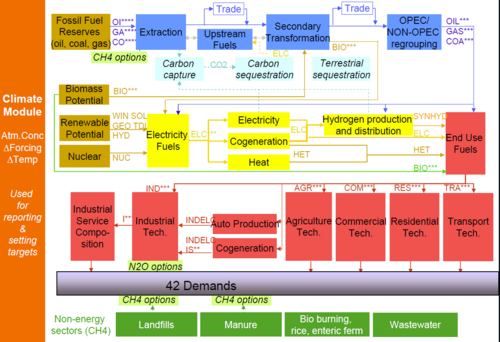
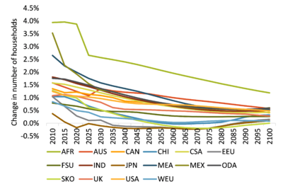
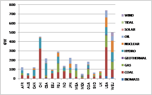
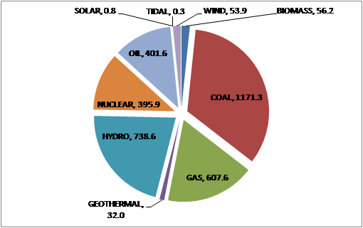
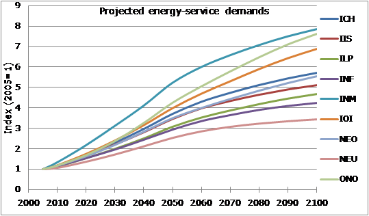
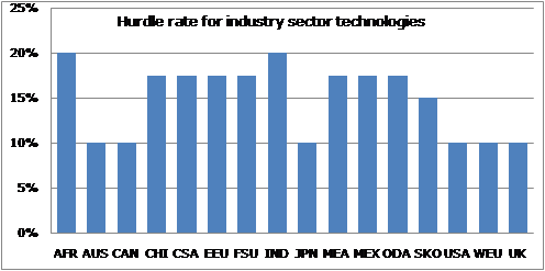
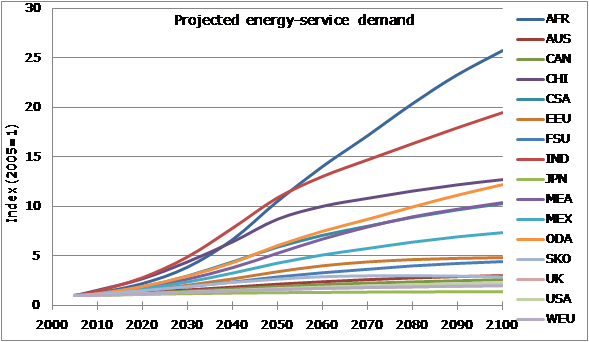
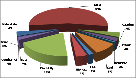
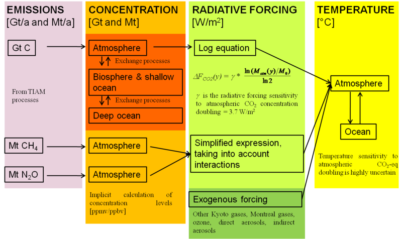
Note: Year divided to six time slices + an additional peaking constraint.