|
|
| Line 25: |
Line 25: |
|
| |
|
| Transfers are determined such that the public administration budget is at equilibrium each year. Public debt is not accounted for. | | Transfers are determined such that the public administration budget is at equilibrium each year. Public debt is not accounted for. |
|
| |
| === Productive sectors ===
| |
|
| |
| A start point for IMACLIM is the recognition that it is almost impossible to find mathematical functions that can handle large departures from a reference equilibrium over a time period of one century and are flexible enough to encompass different scenarios of structural change resulting from the interplay between consumption styles, technologies and localization patterns (Hourcade, 1993)[[CiteRef::hourcade1993modelling]].
| |
|
| |
| ==== Beyond the classical production function, or reconciling bottom-up and top-down approaches ====
| |
|
| |
| In IMACLIM-R, there is no production function, such as a constant elasticity of substitution function, to represent evolutions in production techniques (substitutions between production factors). Instead, evolutions in production techniques are represented in a recursive structure by an exchange of information between static and dynamic modules described as follows:
| |
|
| |
| * An annual static equilibrium module, in which the production function mimics the Leontief specification, with fixed equipment stocks and fixed intensity of labor, energy and other intermediary inputs, but with a flexible utilization rate. Solving this equilibrium at time, ''t'', provides a snapshot of the economy at this date showing a set of information about relative prices, levels of output, physical flows and profitability rates for each sector and allocation of investments among sectors.
| |
|
| |
| * Dynamic modules, including demography, capital dynamics and sector-specific reduced forms of technology-rich models, which take into account the economic values of the previous static equilibrium, assess the reaction of technical systems and send back this information to the static module in the form of new input-output coefficients for calculating the equilibrium at time, 't' + 1. Each year, technical choices are flexible but they modify only at the margin the input-output coefficients and labor productivity embodied in the existing equipment that result from past technical choices. This general putty-clay assumption is critical to represent the inertia in technical systems and the role of volatility in economic signals.
| |
|
| |
| This modelling approach allows for abandoning standard aggregate production functions, which have intrinsic limitations in cases of large departures from the reference equilibrium (Frondel et al., 2002)[[CiteRef::frondel2002capital]] and sea changes of production frontiers over several decades.
| |
|
| |
| As we move away from using a traditional production function, it becomes possible to highlight the influence of factors other than price on decisions affecting the allocation of resources. The use of this modeling approach requires however a comprehensive description of the temporally evolving technical characteristics of each sector.
| |
|
| |
| At each point in time, producers are assumed to operate under constraint of a fixed production capacity ''Cap<sub>k,i</sub>'', defined as the maximum level of physical output achievable with their installed equipment.
| |
|
| |
| However, the model allows short-run adjustments to market conditions through the modification of the utilization rate ''Q<sub>k,i</sub>/Cap<sub>k,i</sub>''. This represents a different approach from standard production specifications, since in Imaclim the 'capital' factor is not always fully utilized. Supply cost curves in Imaclim-R thus show static decreasing returns: production costs increase when the utilization rate of equipment approaches 1 (100 %) (See <xr id="fig:imaclim_4"/>). In principle, these decreasing returns affect all intermediary inputs and labor. However, for the sake of simplicity and because of the order of magnitude of the correlation between utilization rates and prices (Corrado and Mattey, 1997)[[CiteRef::corrado1997capacity]], we assume that the primary cause of higher production costs is higher labor costs due to overtime operations with lower productivity, costly night work and increased maintenance works. We thus set (i) fixed input-output coefficients representing that, with the current set of embodied techniques, producing one unit of good ''i'' in region ''k'' requires the fixed physical amount ''IC<sub>j,i,k</sub>'' of intermediate goods j and ''l<sub>k,i</sub>''of labor; (ii) a decreasing return parameter ''Ω<sub>k,i</sub>= Ω(Q<sub>k,i</sub>/Cap<sub>k,i</sub>)'' on wages only, at the sector level. The treatment of the cost of crude oil production is an exception. The increasing factor weighs on the mark-up rate, to convey the fact that oligopolistic producers can take advantage of capacity shortages by increasing their differential rent.
| |
|
| |
| This solution actually comes back to earlier works on the existence of short-run flexibility of production systems at the sectoral level with putty-clay technologies (Marshall, 1890)[[CiteRef::marshallpoe]], (Johansen, 1959)[[CiteRef::johansen1959substitution]] demonstrating that this flexibility comes less from input substitution than from variations in differentiated capacity utilization rates.
| |
|
| |
| <figure id="fig:imaclim_4">
| |
| [[File:36405273.png|none|600px|thumb|<caption> Sectoral interaction in the Imaclim-R hybrid model</caption>]]
| |
| </figure>
| |
|
| |
| ===== Equations =====
| |
|
| |
| We derive an expression of mean production costs ''Cm<sub>k,i</sub>'', that depends on the prices of intermediate goods ''pIC<sub>j,i,k</sub>'', input-ouput coefficients ''IC<sub>j,i,k</sub>'' and ''l<sub>k,i</sub>'', wages ''w<sub>k,i</sub>'', and production levels through the decreasing return factor ''Ω<sub>k,i</sub>'' applied to labor costs (including payroll taxes).
| |
|
| |
| [[File:36405274.png]]
| |
|
| |
| Market prices and associated profits depend on assumptions regarding the degree of market competition in each sector (e.g. perfect competition or monopoly). Unless otherwise stated, perfect competition is assumed in every production sector, with the market price equal to the marginal production cost.
| |
|
| |
| Producer prices are equal to the sum of mean production costs and mean profits. In the current version of the model, all sectors apply a constant sector-specific mark-up rate ''p<sub>k,i</sub>'' so that the producer price is given by equation (2). This constant mark-up corresponds to a standard profit-maximization for producers whose mean production costs follow equation (1) and who are price-takers, provided that the decreasing return factor can be approximated by an exponential function of utilization rate.
| |
|
| |
| [[File:36405275.png]]
| |
|
| |
| This equation is an inverse supply curve: it shows how a representative producer decides their level of output ''Q<sub>k,i</sub>'' (which is included in the ''Ω<sub>k,i</sub>''factor) as a function of all prices and real wages.
| |
|
| |
| From equation (2) we derive wages and profits in each sector:
| |
|
| |
| [[File:36405276.png]]
| |
|
| |
| The cost function shows fixed technical coefficients and therefore does not allow for substitution between production factors when relative prices change within the new static equilibrium. Only the level of output ''Q<sub>k,i </sub>'' can be adjusted according to these price changes.
| |
|
| |
|
| === Markets === | | === Markets === |
| Line 93: |
Line 47: |
|
| |
|
| A further parameter for the oil sector is that Middle-Eastern producers are considered 'swing producers' who are free to strategically set their investment decisions and, until they reach their depletion constraints, to control oil prices through the utilization rate of their production capacities (Kaufmann et al, 2004)[[CiteRef::kaufmann2004does]]. This possibility is justified by the temporary reinforcement of their market power due to the stagnation and decline of conventional oil in the rest of the world. They can in particular decide to slow the development of production capacities below its maximum rate in order to adjust the oil price according to their rent-seeking objectives. They anticipate the level of capacities that will make it possible for them to reach their goals, on the basis of projections of total oil demand and production in other regions. | | A further parameter for the oil sector is that Middle-Eastern producers are considered 'swing producers' who are free to strategically set their investment decisions and, until they reach their depletion constraints, to control oil prices through the utilization rate of their production capacities (Kaufmann et al, 2004)[[CiteRef::kaufmann2004does]]. This possibility is justified by the temporary reinforcement of their market power due to the stagnation and decline of conventional oil in the rest of the world. They can in particular decide to slow the development of production capacities below its maximum rate in order to adjust the oil price according to their rent-seeking objectives. They anticipate the level of capacities that will make it possible for them to reach their goals, on the basis of projections of total oil demand and production in other regions. |
|
| |
| ==== Capital markets ====
| |
|
| |
| A share (''shareExpK'') of gross domestic savings (GRB) is internationally tradable, and distributed via an international capital pool. Each regions receives a share of the international pool (''shareImpK)''. In the default model setting, both shares (''shareExpK and shareImpK'') are exogenous: ''shareExpK'' is exponentially reduced such that international financial imbalances disappear by 2050 and ''shareImpK'' remains constant throughout the simulation period.
| |
|
| |
| The remaining share of domestic savings and imported capital (NRB) are then invested in each region respectively.
| |
|
| |
| [[File:36405279.png]] ''' (7,8,9)'''
| |
|
| |
| The total amount of money ''InvFin<sub>k,i</sub>'' available for investment in sector ''i'' in the region ''k'' allows new capacities ''DCap<sub>k,i</sub>'' to be constructed at a cost ''pCap<sub>k,i</sub>'' (equation 9-3-5). The cost ''pCap<sub>k,i</sub>'' depends on the quantities ''β<sub>j,i,k</sub>'' and the prices ''pI<sub>k,j</sub>'' of goods ''j'' required by the construction of a new unit of capacity in sector ''i'' and in region ''k''. Coefficient ''β<sub>j,i,k</sub>'' is the amount of good ''j'' necessary to constuct the equipment corresponding to one new unit of production capacity in sector i of the region k. Finally, in each region, the total demand for goods for building new capacities is given by the last equation below.
| |
|
| |
| [[File:36405280.png]]''' (10,11,12)'''
| |
|
| |
| Each sector anticipates future production levels through an anticipation of future prices and demand and formulates the corresponding investment demand. Total available investment ''I<sub>k,j</sub>'' is then distributed among sectors according to their demand.
| |
|
| |
| ==== Labour markets ====
| |
|
| |
| At each time step, producers operate in static equilibria with a fixed input of labor per unit of output. This labor input, corresponding to labor productivity, evolves between two yearly equilibria following exogenous trends in labor productivity.
| |
|
| |
| Three of the model features explain the possibility of under-utilization of labor as a factor of production, and thus unemployment. First, rigidity of real wages, represented by a wage curve can prevent wages falling to their market-clearing level. Put another way, instantaneous adjustment of wages to the economic context in the static equilibrium does not occur in an optimal manner. Second, in the static equilibrium, the fixed technologies (Leontief coefficients even for labor input) prevent substitution among production factors in the short run. And third, the installed productive capital is not mobile across sectors, which creates rigidities in the reallocations of production between sectors when relative prices change.
| |
|
| |
| In each region ''k'', each sector employs the labor force ''l<sub>k,i</sub><sup>.</sup>Q<sub>k,i</sub>'', where ''l<sub>k,i</sub>'' is the unitary labor input (in hours worked) and Q<sub>k,i</sub> the production. The underutilization of the labor force, equivalently referred to as the 'unemployment rate' [2] in the following, ''_z<sub>k</sub>'' is therefore equal to one minus the ratio of the employed labor force across all sectors over ''L<sub>k</sub>'', the total labor force:
| |
|
| |
| [[File:36405281.png]] ''' (13)'''
| |
|
| |
| Obviously, this definition of the unemployment rate is a limitation of the current calibration of the model. Future developments will look into the possibility to differentiate labor markets per regions. However, one important difficulty lies in the lack of reliable data on the underutilization of the labor forces in all regions, in particular due to informal economy, very diverse accounting rules for unemployment rates and variations in hours worked per person across countries. No endogenous mobility of workers between regions is accounted for in the model. Thus twelve separate labor markets are represented.
| |
|
| |
| We chose to model labor market imperfections through an aggregate regional ''wage curve'' that links real wage levels to the unemployment rate. This representation is based on labor theories developed in the 1980s and early 1990s in which an aggregate wage curve, or ''wage setting curve'', is the primary distinguishing feature (an overview can be found in Layard et al., 2005[[CiteRef::layard2005unemployment]]; Lindbeck, 1993[[CiteRef::lindbeck1993unemployment]]; or Phelps, 1992[[CiteRef::phelps1992consumer]]). The novel approach of these models, when introduced, was to replace the conventional labor supply curve with a negatively-sloped curve linking the level of wages to the level of unemployment. The interpretation of this wage curve is given either by the bargaining approach (Layard and Nickell, 1986)[[CiteRef::layard1986unemployment]] or the wage-efficiency approach (Shapiro and Stiglitz, 1984)[[CiteRef::shapiro1984equilibrium]]. Both interpretations rely on the fact that unemployment represents an outside threat that leads workers to accept lower wages the greater the threat. The bargaining approach emphasizes the role of workers' (or union) power in the wage setting negotiations, power that is weakened when unemployment is high. The wage-efficiency approach takes the firms' point of view and assumes that firms set wage levels so as to discourage shirking; this level is lower when the threat of not finding a job after being caught shirking gets higher. The wage curve specification allows the theories to be consistent with both involuntary unemployment and the fact that real wages fluctuate less than the theory of the conventional flexible labor supply curve predicts. Microeconometric evidence for such formulations was given in a seminal contribution by (Blanchflower and Oswald 1995)[[CiteRef::blanchflower1994introduction]].
| |
|
| |
| In practice, the wage curve for each region k in our model is implemented through the relation:
| |
|
| |
| [[File:36405282.png]]''' (14)'''
| |
|
| |
| where ''w'' is the hourly nominal wage level, ''pind'' the consumption price index, ''z'' the unemployment rate, ''ref'' indexes represent the values of the variables at the calibration date, ''pindref'' is derived from the final consumption prices and volumes at the calibration date, ''wref'' is calibrated from the total salaries per sector in the GTAP 6 database (Reference?) and the shares of labor force per sector are taken from International Labor Organisation statistics. By default, ''aw'' is calibrated to 1 and evolves in parallel to labor productivity so that unitary real wages are indexed on labor productivity. ''zref'' represents the underutilization of the labor force at the calibration date. ''f'' is a function equal to one when the unemployment rate is equal to its calibration level, and is negatively sloped, representing a negative elasticity of wages level to unemployment [3]. Choosing a functional form and calibrating the function is particularly tricky, notably due to the lack of reliable data to fully inform the functioning of the labor markets worldwide. We chose a function of the form a.(1-tanh(c.z)), and calibrate the parameters a and c so as to have the desired value and elasticity at the calibration point.
| |
|
| |
| By default, we assume all regions' labor markets to be identical and set the underutilization of the labor force at 10% (Contrary to the definition by the U.S. Bureau of Labor Statistics, the level of unemployment is expressed here in terms of worked hours and not in terms of persons)[4] and the wage curve elasticity at -0.1 for all regions (This is a value emerging from many econometric studies, e.g. (Blanchflower and Oswald 1995)[[CiteRef::blanchflower1994introduction]], (Blanchflower and Oswald 2005). [http://halshs.archives-ouvertes.fr/docs/00/72/44/87/PDF/Guivarch_et_al_2011_Costs_climate_policies_second_best_world_labour_market_imperfections.pdf Guivarch et al. (2011)][[CiteRef::guivarch2011costs]] analyzes the critical role of labour markets imperfections, and in particular of the value of the wage curve elasticity, on the formation of climate stabilization costs.
| |
|
| |
| === International Trade ===
| |
|
| |
| For each good, exports from all world regions are blended into an international variety, which is then imported by each region based on its specific terms-of-trade measured between the price of the aggregate international variety, and the production price of the domestic good.
| |
|
| |
| International trade is treated 'upstream': the competition of the domestic and imported varieties of each good is settled in an aggregate manner, not at the level of each domestic agent.
| |
|
| |
| A well-known modelling issue is then to avoid 'knife-edge' solutions, ''i.e.'' to prevent cheaper goods systematically winning market shares over more expensive ones. We follow the most common approach to addressing this issue, the Armington (1969)[[CiteRef::sassi2010im]] specification, which assumes that the domestic and imported varieties of the same good aggregate in a common quantity index, although in an imperfectly substitutable way which is typically derived from assuming that the two varieties combine through a constant elasticity of substitution (CES) function. This allows representing markets in which both domestic production and imports have a share, despite the fact that they are priced differently.
| |
|
| |
| Despite its straightforward treatment of imperfect product competition, the Armington specification has the major drawback of introducing aggregate volumes that do not sum up the volumes of imported and domestic varieties. While this shortcoming can be ignored for non-descript 'composite' goods, where quantity units are indexes of no direct significance to the economy-energy-environment interactions, it is not compatible with the obvious need to track energy balances expressed in real physical units. Competition between energy goods is thus settled through simplified specifications. In the case of national models, the hypothesis of a constant elasticity of substitution is retained, but the construction of a composite index is dropped. Imports and domestic production are simply summed up to form the resource that is available to the importing economy. For the multi-regional version of Imaclim, a market-sharing formula is implemented. The international market buys energy exports at different prices and sells them at a single average world price to importers; shares of exporters on the international market and regional shares of domestic ''vs.'' imported energy goods dependent on relative prices, export and import taxes, and market fragmentation parameters that are calibrated to reproduce the existing markets structure.
| |
|
| |
| For all goods, export prices include the producer prices, export taxes or subsidies, and average transportation costs. This allows the model to take into account that increasing energy prices would impact on transportation costs and eventually on commercial flows and industrial location patterns.
| |
|
| |
| ''Armington goods'' [[File:36405284.png]]''' (15,16,17)'''
| |
| [[File:36405285.png]]''' (18,19,20)'''
| |
| [[File:36405286.png]]''' (21,22)'''
| |
|
| |
| ''Energy goods''
| |
|
| |
| [[File:36405287.png]]''' (23,24,25)'''
| |
| [[File:36405288.png]]''' (26,27,28)'''
| |
| [[File:36405289.png]]''' (29,30,31)'''
| |
|
| |
|
| |
| -----
| |
|
| |
| [1] The treatment of the cost of crude oil production is an exception. The increasing factor weighs on the mark-up rate, to convey the fact that oligopolistic producers can take advantage of capacity shortages by increasing their differential rent.
| |
|
| |
| [2] Obviously, this is a limitation of the current calibration of the model. Future developments will look into the possibility to differentiate labor markets per regions. However, one important difficulty lies in the lack of reliable data on the underutilization of the labor forces in all regions, in particular due to informal economy, very diverse accounting rules for unemployment rates and variations in hours worked per person across countries.
| |
|
| |
| [3] Choosing a functional form and calibrating the function is particularly tricky, notably due to the lack of reliable data to fully inform the functioning of the labor markets worldwide. We chose a function of the form a.(1-tanh(c.z)), and calibrate the parameters a and c so as to have the desired value and elasticity at the calibration point.
| |
|
| |
| [4] Contrary to the definition by the U.S. Bureau of Labor Statistics, the level of unemployment is expressed here in terms of worked hours and not in terms of persons.
| |
|
Model Documentation - IMACLIM
|
|
|
| Corresponding documentation
|
|
|
| Previous versions
|
|
|
| Model information
|
| Model link
|
|
| Institution
|
Centre international de recherche sur l'environnement et le développement (CIRED), France, http://www.centre-cired.fr., Societe de Mathematiques Appliquees et de Sciences Humaines (SMASH), France, http://www.smash.fr.
|
| Solution concept
|
General equilibrium (closed economy)
|
| Solution method
|
SimulationImaclim-R is implemented in Scilab, and uses the fonction fsolve from a shared C++ library to solve the static equilibrium system of non-linear equations.
|
| Anticipation
|
Recursive dynamics: each year the equilibrium is solved (system of non-linear equations), in between two years parameters to the equilibrium evolve according to specified functions.
|
A general equilibrium with rigidities
The representation of the economy in Imaclim-R is a multi-sector (12 sectors), multi-region (12 regions) general equilibrium framework. In each region, there are 14 economic agents: one representative household, one representative firm per sector (hence 12 representative firms) and the public administration. Households receive revenues from labor and capital and from transfers from public administrations and save part of their revenues. They chose their consumptions of goods and services depending on relative prices and they pay taxes to the public administrations. Productive sectors chose their production levels to meet demand, earn profits, pay wages and dividends to households and pay taxes to public administrations. Public administrations collect taxes, make public expenditures and invest in public infrastructures, and organize transfers. Regions are linked through international markets for goods and services, and capital. <xr id="fig:imaclim_3"/> outlines these interrelationships.
<figure id="fig:imaclim_3">
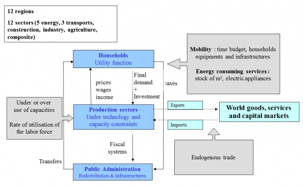
Sectoral interaction in the Imaclim-R hybrid model
</figure>
Households
Each year, households maximize their current utility under constraints of both revenue received and of their time spent in transport. They save an exogenous share of their revenues. For detailed descriptions of demand formation mechanisms refer to the section on demand representation.
Public administrations
Public administrations collect taxes, make public expenditures including investment in public infrastructures and organize transfers.
Tax rates (and/or subsidies) are calibrated to their values for the model calibration year (2001). Taxes (and/or subsidies) impact upon energy, labor, revenues, added value, production, imports and exports. In the default setting of the model, tax rates are kept constant throughout the modelling period (except for in scenarios that model the introduction of a carbon tax ) although alternative assumption on tax rates can also be tested. In a scenario where a carbon tax is introduced, alternative assumptions on the use of the corresponding revenues can be modelled i.e. they are given to households via transfers, used to reduce other pre-existing tax rates or used to finance a subsidy.
In the default setting public expenditures in each region are assumed to follow GDP growth rates, Alternative assumptions on the evolution of public expenditures can also be tested.
Transfers are determined such that the public administration budget is at equilibrium each year. Public debt is not accounted for.
Markets
Markets of goods and services
In the Imaclim-R model, all intermediate and final goods are internationally tradable and total demand for each good (the sum of households' consumption, public and private investments and intermediate uses) is satisfied by a mix of domestic production and imports (see section on international trade XXXXXXXXXXXXXXXXX). Domestic as well as international markets for all goods are cleared (i.e. no stock is allowed) by a unique set of relative prices calculated in the static equilibrium such that demand and supply are equal.
Price
In each region k and sector i, the price equation is:
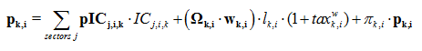 (5)
(5)
where πk,i is a markup, ICj,i,k are intermediate consumption of good j in sector i in region k, and Ωk,i is an increasing cost (or decreasing returns) function of the productive capacities utilization rate. This function is applied to labor costs (which include wages wk,i and labor taxes taxk,i).
The functional form for Ω is:
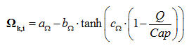 (6)
(6)
Regional prices thus correspond to the addition of average regional production costs and a margin. This markup, which is fixed in the static equilibrium, encapsulates Ricardian and scarcity rents at the same time and increases with the utilization rate of production capacities in the oil sector.
A further parameter for the oil sector is that Middle-Eastern producers are considered 'swing producers' who are free to strategically set their investment decisions and, until they reach their depletion constraints, to control oil prices through the utilization rate of their production capacities (Kaufmann et al, 2004)kaufmann2004does. This possibility is justified by the temporary reinforcement of their market power due to the stagnation and decline of conventional oil in the rest of the world. They can in particular decide to slow the development of production capacities below its maximum rate in order to adjust the oil price according to their rent-seeking objectives. They anticipate the level of capacities that will make it possible for them to reach their goals, on the basis of projections of total oil demand and production in other regions.

 (5)
(5)
 (6)
(6)